Todays topics:
Chain rule:
- Composite functions: They are functions that are composed of another functions, for example: $F(x) = f(g(x))$. Chain rule can be used to derivate these types of functions
- The above is a simple case, we can just say that the internal function be like y = $f(x)$ then $x= g(t)$. So finally we get $\frac{dy}{dt} = \frac{dy}{dx} \cdot \frac{dx}{dt}$
- There are other cases depending on the number of variables in the function.
- Case 1: $z = f(x,y), x = g(t), y = h(t)$, we need to find the ratio $\frac{dz}{dt}$
- Since the connection between independent and dependent variable is direct, we can use the form similar to above
- $\frac{dz}{dt}=\frac{\partial{f}}{\partial{x}} \cdot\frac{dx}{dt} + \frac{\partial{f}}{\partial{y}} \cdot \frac{dy}{dt}$
- Case 2: $z=f(x,y);x=g(s,t)and y=h(s,t)$ Here the internal function has two variables in them, so the goal here becomes finding two ratios $\frac{\partial{z}}{\partial{s}} \& \frac{\partial{z}}{\partial{t}}$
- We can use a tree diagram to find all the components of differential function.
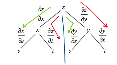
- The first two branches becomes the immediat variables inside the main function. Then in the second layer the internal functions can be further divided into their own independent variables.
- At the end we add allthe partial derivatives together which gives the final ratio.
Vector fields and Gradients:
- A gradient is fancy word for a derivative or rate of change of function. A vector that points in the direction of greatest(steepest) change of a function
- A vector field is also called as ‘gradient vector field. So , a vector field in 2D or 3D is a function $\overrightarrow{F}$. It assigns a 2D or 3D vector to each point in the space.
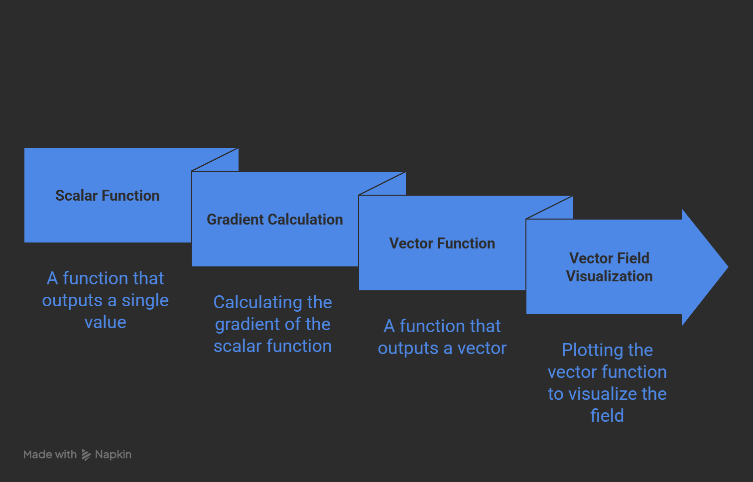
- Scalar functions and Vector functions!! When the function taht outputs scalars then it is a scalar function. When the output is vector, then it is a vector function.
- Now For a scalar function $f(x,y,z)$ the vector function becomes $\nabla{f} = <f_x,f_y,f_z>$. The terms inside the vector function are the partial derivatives of the function f wrt (x,y,z). They are also called as vector components.
- \[\nabla{f}= \begin{bmatrix} f_x \\ f_y \\ f_z \end{bmatrix} = f_x\overrightarrow{i}+f_y\overrightarrow{j}+f_z\overrightarrow{z}\]
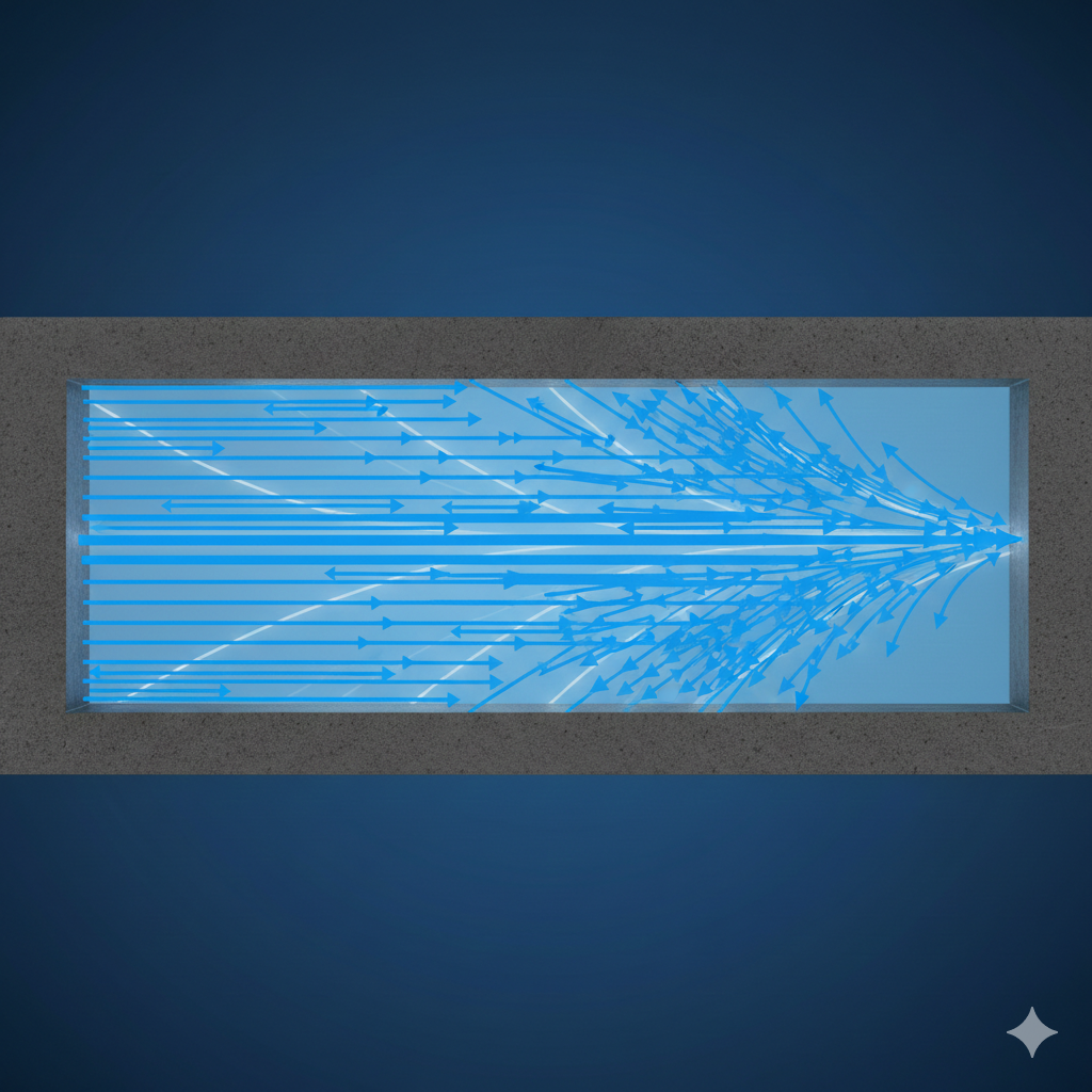
- An example of vector field is the flow of fluid inside a pipe
- An example take the function $f(x,y) = x^2 sin(5y)$. Then the vector field becomes $\nabla{f} = <2xsin(5y), 5x^2cos(5y)>$.
- We can substitue the x and y values to the vector function to get the directional vector for that point in the space representing the biggest change in the function.
Directional derivatives:
- A directional derivative is the rate of change of function in a given direction. In another words, given a direction, the quantity of change of functions in given by directional derivative.
- In the previous chapter we saw that the maximum change in the function is given by the gradient, so it would be common sense to think that the directional derivative would be maximum when the directional derivative points towards the gradient.
- We can prove this using dot product properties:
- Given a function f(x,y) and a unit vector $\overrightarrow{u} = <a,b>$ then the directional derivative is represented as $D_\dot{u}f(x,y)$
- The directinal derivative is given as \(D_\dot{u}f(x,y) = f_x(x,y)a + f_y(x,y)b \implies <f_x, f_y>.<a,b> \iff \begin{bmatrix} f_x \\ f_y \end{bmatrix} \cdot \begin{bmatrix} a \\ b \end{bmatrix}\)
- This above expression boils down to the dot product between the gradient vector function and unit vector for given direction.
- $D_\dot{u}f(x,y) = \nabla{f} \cdot \overrightarrow{u}$
- Then the max value for the $D_\dot{u}f(x,y)$ occurs when the angle between the two vectors is 0. cause $cos(0)=1$ in other words, when the directional vector points towards unit vector.
Jacobian and Hessian Matrices:
- When the function has multiplie independent variables, it could be hard to find the direction of the steepest change in the function.
- One has to look at all the directions(towards all the variables). This is where we get the Jacobian and Hessian Matrices
- Jacobian and Hessian Matrices describe the ‘slope’ and ‘curvature’ of the multi variate function.
Jacobian Matrix:
- Jacobian is a matrix composed of the first-order partial derivatives of the multi variate-vector function.
- For a function $f(x_1,x_2..x_n) = (f_1, f_2,..f_m)$
- The jacobian matrix will have n- columns (as many as the number of vector components) and m- rows (as many as the number of variables)
- \[J_f = \begin{bmatrix} \frac{\partial{f_1}}{\partial{x_1}}&\frac{\partial{f_1}}{\partial{x_2}}&.&.&.&\frac{\partial{f_1}}{\partial{x_n}}\\ \frac{\partial{f_2}}{\partial{x_1}}&\frac{\partial{f_2}}{\partial{x_2}}&.&.&.&\frac{\partial{f_2}}{\partial{x_n}}\\ .&. \\ .&. \\ .&. \\ \frac{\partial{f_m}}{\partial{x_1}}&\frac{\partial{f_m}}{\partial{x_2}}&.&.&.&\frac{\partial{f_m}}{\partial{x_n}} \\ \end{bmatrix}\]
- Uses of Jacobian matrix:
- To approximate the complex multi variate vector function to a linear flat plane around a point ‘P’. The shape of the function can be complex in different dimensions, to find a value at a point P with much lesser computational costs we approximate a function to a linear function around ‘P’.
- The determinant of the Jacobian (Jacobian) tells if the function is ‘locally invertable’
- $det(J)\ne0$, The function is locally invertable
- $det(J)=0$, The function is not invertable
- Apart from these, the Jacobian matrix is helpful in determining critical points. Remember when we equate the first differential to 0 then we are essentially finding the points where the function has a maximum or minimum? It’s the same here, to find these critical points, we equate $J_f(x,y) = 0$ Now solve the system of equations to find the critical points.
- Later these critical points are classified to maximum or minimum with the Hessian Matrix
Hessian Matrix:
- Like Jacobian matrix, Hessian Matrix is made of differentials. However, Hessian Matrix contains ‘second order derivatives’.
- It gives the ‘curvature of the function’.
- Hessian Matrix is a symmetric matrix
- For $f(x,y)$, \(H = \begin{bmatrix} \frac{\partial^2 f}{\partial x^2} & \frac{\partial^2 f}{\partial x \partial y} \\ \frac{\partial^2 f}{\partial y \partial x} & \frac{\partial^2 f}{\partial y^2} \end{bmatrix}\)
- It can be used to find if the point belongs to a pit(Minimum), peak(Maximum) or a mountain passing. For this we find something called Discriminant (D)
- Discriminant (D) = $f_{xx}f_{yy}-f_{xy}^2$
- Then, if $D>0 and f_{xx} <0$ then the P is a local Minimum
- Then, if $D>0 and f_{xx} >0$ then the P is a local Maximum
- Then, if $D<0$ then the P is a Saddle Point. A Saddle point is where one direction curves up and one direction curves down.