<?xml version="1.0" encoding="utf-8"?><feed xmlns="http://www.w3.org/2005/Atom" ><generator uri="https://jekyllrb.com/" version="3.10.0">Jekyll</generator><link href="https://jayadeep19.github.io/til-notes/feed.xml" rel="self" type="application/atom+xml" /><link href="https://jayadeep19.github.io/til-notes/" rel="alternate" type="text/html" /><updated>2026-02-23T22:54:06+00:00</updated><id>https://jayadeep19.github.io/til-notes/feed.xml</id><title type="html">TIL-notes</title><subtitle>Today I learned</subtitle><author><name>Jayadeep</name></author><entry><title type="html">Statistics: Data and Sampling Distributions</title><link href="https://jayadeep19.github.io/til-notes/data-sampling-distribution" rel="alternate" type="text/html" title="Statistics: Data and Sampling Distributions" /><published>2026-02-03T00:00:00+00:00</published><updated>2026-02-03T00:00:00+00:00</updated><id>https://jayadeep19.github.io/til-notes/data-sampling-distribution</id><content type="html" xml:base="https://jayadeep19.github.io/til-notes/data-sampling-distribution"><![CDATA[<p>Today I learned about Sampling and their distributions. When There is huge dataset with unknown distribution, we do not have a good idea what to expect in the patterns in the data. We then take some samples(a subset of the dataset) and make inferences about the true dataset. The true dataset is called as Population and the sample of a population can be represented by $N(n)$.</p>
<ul>
  <li>Sometimes quality is better than quantity. Smaller samples give better description about the data that the population itself. This is one of the reason why a better sampling is required.</li>
</ul>

<p>Todays topics:</p>
<ul id="markdown-toc">
  <li><a href="#sampling" id="markdown-toc-sampling">Sampling</a></li>
  <li><a href="#sampling-distribution-of-a-statistic" id="markdown-toc-sampling-distribution-of-a-statistic">Sampling distribution of a statistic:</a>    <ul>
      <li><a href="#central-limit-theorem" id="markdown-toc-central-limit-theorem">Central Limit Theorem:</a></li>
      <li><a href="#standard-error" id="markdown-toc-standard-error">Standard Error:</a></li>
    </ul>
  </li>
</ul>

<h2 id="sampling">Sampling</h2>
<ul>
  <li>Bias:
    <ul>
      <li>Statistical bias refers to measurement errors or sample errors that are produced by either during measurement or during sampling.</li>
      <li>It is important to differentiate between these two biases and several methods were developed to reduce this sampling bias. One of the method is Random Sampling</li>
    </ul>
  </li>
  <li>The most basic sampling is <strong>Random sampling</strong>. We take a random member of a population to the sample. All the members in the population has an equal chance of getting selected. In selecting the next sample, we can Replace the picked up member back to the population (called as Replacement) or we can leave it out if population for the next samples (without Replacement).
-To achioeve a better representation of the population through sampling, it could be useful to look at questions like:
    <ul>
      <li>Do we need to startify the data into smaller sub groups of data with similar properties before sampling?</li>
      <li>Does assigning weights to different stratified subsets to achieve better sample sizes?
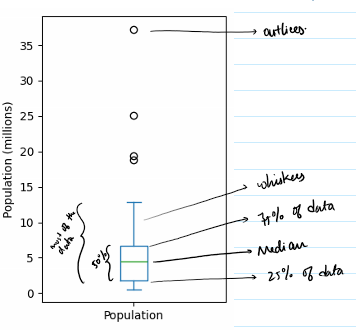
</li>
    </ul>
  </li>
  <li><strong>Sample Means vs Population Means</strong>:
    <ul>
      <li>The mean of the sample($\bar{x}$) is often different from the mean of the population ($\bar{\mu}$).This is important because the variation of the sample means across different samples can give a lot of information about the population.</li>
    </ul>
  </li>
  <li>A normal procedure to model a dataset is:
    <ul>
      <li>To specify a hypothesis (more about this later)</li>
      <li>Conduct a well designed Experiment to test the hypothesis.</li>
      <li>Have results</li>
    </ul>
  </li>
  <li>But this is not what happens in general. The Person modeling the dataset may go on an extensive search through the dataset in search of patterns and sooner or later, there comes a pattern. But the question is, is this really a pattern or just a <em>Data snooping</em>. Another interesting phenomenon is <em>Data Snooping</em>, it occurs when the data is extensively hunted through to find somethong interesting. This leads to</li>
  <li><strong>Selection Bias</strong>:
    <ul>
      <li>When a Datascientist or a statistician selects the samples selectively so that leads to a conclusion is called selection bias.</li>
    </ul>
  </li>
</ul>

<h2 id="sampling-distribution-of-a-statistic">Sampling distribution of a statistic:</h2>
<ul>
  <li>As we discussed above, the distribution of the mean of a sample is important for infering information about the population. So in this section we look closer at sampling distributions</li>
  <li>Sampling metric is a metric calculated foa a sample</li>
  <li>
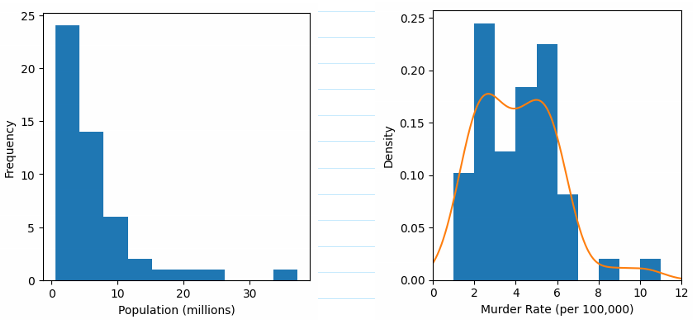
Sampling distribution is the frequency distribution of a sample statistic over several samples. While data distribution is the frequency distribution of the individual data points.</li>
  <li>We can now, try to estimate this sampling distribution to see how far the sample statistic is from the population statistic (eg: mean)</li>
  <li>About Sampling Distribution:
    <ul>
      <li>Sampling distribution of samples resembles bell curve.</li>
      <li>The above statement is governed by <strong>Central Limit Theorem (CLT)</strong></li>
    </ul>
  </li>
</ul>

<h3 id="central-limit-theorem">Central Limit Theorem:</h3>
<ul>
  <li>It states that the means drawn from several samples will resemble a bell curve given:
    <ul>
      <li>The sample size is large enough</li>
      <li>The values of data doesnt depart from normality too much.</li>
      <li>For a data scientist, CLT is not so important but for traditional statistics it is a very important theorem as it lays foundational grounds for Hypothesis testing, confidence intervals.</li>
      <li>A better method called boot strap is always available for estimating sampling distribution that does not assume that the sampling dist forms bell curves. (more on bootstrap later)</li>
    </ul>
  </li>
</ul>

<h3 id="standard-error">Standard Error:</h3>
<ul>
  <li>Population: You have a big, unknown group.</li>
  <li>Samples/Resamples: You take many samples of size $n$.</li>
  <li>Sample Metric: You calculate the mean ($\bar{x}$) for every single sample.</li>
  <li>Sampling Distribution: You plot all those means. Because of the CLT, they form a bell curve</li>
  <li>Now we can calculate the standard deviation of this bell curve to find the spread of the curve or the variability of the sample means</li>
  <li>But, the problem is we do not have to take several thousands of samples to estimate the sampling distribution. We can take one sample and then we can try to estimate ‘Standard Error’ for a sample and scatter it to remaining samples.</li>
  <li>Because, the shape of the curve is ‘bell curve’, we need two inputs for the normal distribution estimation. The mean and the standard deviation. This standard deviation is here called as ‘Standard Error’</li>
  <li>Standard Error is a single metric to measure the variability of sampling distribution.</li>
  <li>It is given by $SE = \frac{s}{\sqrt{n}}$ ; s = <a href="/statistics1#Estimates of Variability:">standard deviation</a></li>
  <li>From the above equation, we can deduce that that:
    <ul>
      <li>As the sample size(n) increases, the Standard error decreases.</li>
      <li>
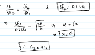
This relation ship btwn SE and Sample size is reffered to as ‘Square root of n’ rule.</li>
      <li>When the SE to go down by a factor of 2 the sample size has to be increased by 4times.</li>
      <li><img src="/til-notes/assets/img/statistics/Standard_error.png" alt="standard-error" /></li>
    </ul>
  </li>
  <li>While this method is useful in estimating SE, it has several con’s:
    <ul>
      <li>Assumption of bell curve for the sampling dist</li>
      <li>The standard deviation of the sample is used for the estimation of SE. if the sample taken is by chance abnormal, this could mess up the SE estimation.</li>
      <li>This method only works for the metric mean.</li>
    </ul>
  </li>
  <li>This method of taking samples and estimating the SE is not efficient in statistical terms(not resourceful). There is another effective method called ‘BOOT STRAP’ method of resampling.</li>
</ul>]]></content><author><name>Jayadeep</name></author><category term="math" /><category term="datascience" /><category term="documentation" /><category term="Feb26" /><summary type="html"><![CDATA[Today I learned about Sampling and their distributions. When There is huge dataset with unknown distribution, we do not have a good idea what to expect in the patterns in the data. We then take some samples(a subset of the dataset) and make inferences about the true dataset. The true dataset is called as Population and the sample of a population can be represented by $N(n)$. Sometimes quality is better than quantity. Smaller samples give better description about the data that the population itself. This is one of the reason why a better sampling is required.]]></summary></entry><entry><title type="html">Statistics: Exploratory data analysis</title><link href="https://jayadeep19.github.io/til-notes/statistics1" rel="alternate" type="text/html" title="Statistics: Exploratory data analysis" /><published>2026-02-01T00:00:00+00:00</published><updated>2026-02-01T00:00:00+00:00</updated><id>https://jayadeep19.github.io/til-notes/statistics1</id><content type="html" xml:base="https://jayadeep19.github.io/til-notes/statistics1"><![CDATA[<ul>
  <li>I have started a new book this month that is named ‘Practical statistics for Data Scientists’.</li>
  <li>Todays topics are mostly from that book. The first chapter is Exploratoty data analysis. Although I know most of these concepts, I would still like to document the learnings for the sake of completness.</li>
  <li>The first steps for any project is analysing the raw data, filtering, and structure the data into a ‘more easy for the machine or algorithm’ way to train a statistical model.</li>
  <li>The structured data could be either
    <ol>
      <li>Numeric: Data Expressed as Numericals
        <ul>
          <li>Continuous :</li>
          <li>Discrete</li>
        </ul>
      </li>
      <li>Categorical: The data takes a set of values (ex types of tv screens: Lcd:1; plasma:2,..)
        <ul>
          <li>Binary: 0 or 1</li>
          <li>Ordinal: Ordered categories.</li>
        </ul>
      </li>
    </ol>
  </li>
  <li>Rectangular data:
    <ul>
      <li>For analysis, the data is mostly organised in a rectangular frame (2D matrix) of reference in most of the softwares like spread sheets ot databases.</li>
      <li>The columns are called as Features that are used to predict a value called target variable.
        <ul>
          <li>To predict weather, we could used features like humidity, windspeed, sunny..</li>
        </ul>
      </li>
      <li>The rows are the records or observations.</li>
      <li>The data could be Non rectangular, like time series data, graph datastructures and so on.. In this blog rectangular data is focused.</li>
    </ul>
  </li>
</ul>

<p>Todays topics:</p>
<ul id="markdown-toc">
  <li><a href="#estimates-of-location" id="markdown-toc-estimates-of-location">Estimates of Location:</a></li>
  <li><a href="#estimates-of-variability" id="markdown-toc-estimates-of-variability">Estimates of Variability:</a></li>
  <li><a href="#exploring-the-data-distribution" id="markdown-toc-exploring-the-data-distribution">Exploring the Data Distribution:</a></li>
  <li><a href="#correlation" id="markdown-toc-correlation">Correlation:</a></li>
  <li><a href="#exploring-two-or-more-variables" id="markdown-toc-exploring-two-or-more-variables">Exploring two or more variables:</a></li>
</ul>

<h2 id="estimates-of-location">Estimates of Location:</h2>
<ul>
  <li>When there are 1000’s of observations for a feature, It might be a good start for the anaysis to know where most of the observations lie. For example: most of the observations for Humidity is around $25^0$.</li>
  <li>The metrics used to estimate the location for a feature are as follows:</li>
  <li><strong>Mean</strong>:
    <ul>
      <li>The avreage value of all the observations</li>
      <li>$mean(\bar{x} = \frac{\sum_1^n{x_i}}{n})$</li>
      <li>Note: the mean is very sensitive to outliers(extreme values in the observations). So there are other better metrics for estimating location.</li>
      <li><strong>Trimmed Mean</strong>:
        <ul>
          <li>Before calculating the mean, the extreme values are trimmed/dropped.</li>
          <li>Instead of ‘n’ observations we substract ‘p’ largest and ‘p’ smallest values in the observations</li>
          <li>This essentially reduces the sensitivity to extreme values.</li>
        </ul>
      </li>
      <li><strong>Weighted Mean</strong>:
        <ul>
          <li>We can multiply each datapoint($x_i$) with a specific weight to tweek the individual influence of a datapoint on the final value.</li>
          <li>$\bar{x_w} = \frac{\sum_1^n{w_ix_i}}{\sum_1^n{w_i}}$</li>
          <li>This method is useful in cases where the proportion of observations for two categories are not similar. We can assign a higher weight to the group with less number of observations. This reduces the bias towards the group with larger data points/observations.
-<strong>Median</strong>:</li>
        </ul>
      </li>
      <li>The middle value in a sorted data is called ti median of the data.</li>
      <li>When there are even number of datapoints, we take the average of both the middle values</li>
      <li>Median is robust to outliers</li>
    </ul>
  </li>
</ul>

<blockquote>
  <p>Outliers are sometimes informative and sometimes nuisance. Anamoly detection is used to determine the outliers, I will get to this in a later blog.</p>
</blockquote>

<h2 id="estimates-of-variability">Estimates of Variability:</h2>
<ul>
  <li>In the next step of exploring the data, one might be interested in finding how spread out the data is.</li>
  <li>The various metrics for measuring variability are:
    <ul>
      <li><strong>Deviation</strong>:
        <ul>
          <li>The difference between Observed and the estimate of location.</li>
          <li>We can then take the mean of these deviations for the absolute values(without the sign of the deviation) from the mean is called mean absolute deviation</li>
          <li>$Mean\ absolute\ deviation = \frac{\sum{|x_i-x|}}{n}$</li>
        </ul>
      </li>
      <li><strong>Variance</strong>:
        <ul>
          <li>Variance is the average of the squared deviations.</li>
          <li>Following the Variance is the important metric <strong>standard deviation</strong>. It is the square root of the variance.</li>
          <li>$Variance = s^2 = \frac{\sum{(x_i-\bar{x})^2}}{n-1}$</li>
          <li>the denominator is not n because of something called ‘degrees of freedom’. As n is a large number, when taken ‘n-1’ as denominator it would not make much difference and also it reduces the redundency in data during the calculation of variance.</li>
          <li>Then the $Standard\ Deviation$ is given by $s = \sqrt{variance}$</li>
        </ul>
      </li>
    </ul>
  </li>
  <li>The standard deviation is mostly used metric because, it lies in the same dimension as the data.
    <ul>
      <li>These metrics are not robust to outliers, A more robust metric would be ‘Median Absolute Deviation from the median’.
        <ul>
          <li>$MAD = median(|x_1-m|, |x_2-m|,…|x_n-m|)$</li>
        </ul>
      </li>
      <li>Percentile Extimate:
        <ul>
          <li>Percentile is a value below which a certain percentage of the datafalls. For example, $p^th$ percentile is a value for which atleast p percentage of the values has observed value lesser this value and (100-p) percentile takes on value greater than this value.</li>
          <li>For example, 90th percentile for height menas that I am taller than 90% of the people in the dataset.</li>
          <li>This is where we have the concept of <em>Inter Quartile Range(IQR)</em> The dataset is divided int0 4 quartiles.</li>
          <li>1st Quartile- 25th percentile</li>
          <li>2nd Quartile- 50th percentile</li>
          <li>3rd Quartile- 75th percentile</li>
          <li>4th Quartile- 100th percentile</li>
          <li>The IQR is then $Q_3-Q_1$. Basically we consider the 50% of data in the middle of the dataset.</li>
        </ul>
      </li>
    </ul>
  </li>
</ul>

<h2 id="exploring-the-data-distribution">Exploring the Data Distribution:</h2>
<ul>
  <li>Instead of summarizing the data into a single number to make some initial sense of the data, we can see visually how the data is distibuted.</li>
  <li>Several plots are developed by statistians to visualise the spread of the data.</li>
  <li>Box plots:
    <ul>
      <li>These are based on the percentile we discussed above.</li>
      <li>The plot indicates outliers, and the 4 quartiles along with the IQR of the data.</li>
      <li><img src="/til-notes/assets/img/statistics/boxplot.png" alt="boxplot" /></li>
    </ul>
  </li>
  <li>Frequency tables, histograms and density plots:
    <ul>
      <li>The data is classified into bins and the count in each bin is called the frequency of the bin.</li>
      <li>We can use a histogram to visualise the data.</li>
      <li>For a density plot we can use a ‘kernal density estimate’ to smoothen the histogram
  <img src="/til-notes/assets/img/statistics/histogram.png" alt="boxplot" /></li>
    </ul>
  </li>
</ul>

<h2 id="correlation">Correlation:</h2>
<ul>
  <li>In Exploratory data analysis, one of the important concept is to check for correlation.</li>
  <li>Correlation is measuring the relation between two predictors or between predictor and target.</li>
  <li>Say two features x,y. How does y change when the x changes. This measure is called correlation.</li>
  <li>Correlation coefficient is metric used to measure the correlation between two features. Its value lies between (-1 and 1). -1 indicates lower correlation and 1 indicating higher correlation between features.
    <ul>
      <li>Pearson Correlation Coefficient: $\frac{\sum{(x_i-\bar{x})(y_i-\bar{y})}}{(n-1)s_xs_y}$</li>
    </ul>
  </li>
  <li>When the relation between features are not linear, correlation may not be an important metric.</li>
  <li>This above method of correlation is not robust to outliers.</li>
</ul>

<h2 id="exploring-two-or-more-variables">Exploring two or more variables:</h2>
<ul>
  <li>Some of the plot can be used to explore two or more variables simultaneously.
    <ol>
      <li>Contingency table</li>
      <li>Hexagonal binning</li>
      <li>Contour plots</li>
      <li>Violin plot.</li>
    </ol>
  </li>
</ul>]]></content><author><name>Jayadeep</name></author><category term="math" /><category term="datascience" /><category term="documentation" /><category term="Feb26" /><summary type="html"><![CDATA[I have started a new book this month that is named ‘Practical statistics for Data Scientists’. Todays topics are mostly from that book. The first chapter is Exploratoty data analysis. Although I know most of these concepts, I would still like to document the learnings for the sake of completness. The first steps for any project is analysing the raw data, filtering, and structure the data into a ‘more easy for the machine or algorithm’ way to train a statistical model. The structured data could be either Numeric: Data Expressed as Numericals Continuous : Discrete Categorical: The data takes a set of values (ex types of tv screens: Lcd:1; plasma:2,..) Binary: 0 or 1 Ordinal: Ordered categories. Rectangular data: For analysis, the data is mostly organised in a rectangular frame (2D matrix) of reference in most of the softwares like spread sheets ot databases. The columns are called as Features that are used to predict a value called target variable. To predict weather, we could used features like humidity, windspeed, sunny.. The rows are the records or observations. The data could be Non rectangular, like time series data, graph datastructures and so on.. In this blog rectangular data is focused.]]></summary></entry><entry><title type="html">Vector calculus</title><link href="https://jayadeep19.github.io/til-notes/vector-calculus" rel="alternate" type="text/html" title="Vector calculus" /><published>2026-01-23T00:00:00+00:00</published><updated>2026-01-23T00:00:00+00:00</updated><id>https://jayadeep19.github.io/til-notes/vector-calculus</id><content type="html" xml:base="https://jayadeep19.github.io/til-notes/vector-calculus"><![CDATA[<p>Todays topics:</p>
<ul id="markdown-toc">
  <li><a href="#chain-rule" id="markdown-toc-chain-rule">Chain rule:</a></li>
  <li><a href="#vector-fields-and-gradients" id="markdown-toc-vector-fields-and-gradients">Vector fields and Gradients:</a></li>
  <li><a href="#directional-derivatives" id="markdown-toc-directional-derivatives">Directional derivatives:</a></li>
  <li><a href="#jacobian-and-hessian-matrices" id="markdown-toc-jacobian-and-hessian-matrices">Jacobian and Hessian Matrices:</a>    <ul>
      <li><a href="#jacobian-matrix" id="markdown-toc-jacobian-matrix">Jacobian Matrix:</a></li>
      <li><a href="#hessian-matrix" id="markdown-toc-hessian-matrix">Hessian Matrix:</a></li>
    </ul>
  </li>
</ul>

<h2 id="chain-rule">Chain rule:</h2>
<ul>
  <li>Composite functions: They are functions that are composed of another functions, for example: $F(x) = f(g(x))$. Chain rule can be used to derivate these types of functions</li>
  <li>The above is a simple case, we can just say that the internal function be like y = $f(x)$ then $x= g(t)$. So finally we get $\frac{dy}{dt} = \frac{dy}{dx} \cdot \frac{dx}{dt}$</li>
  <li>There are other cases depending on the number of variables in the function.
    <ol>
      <li>Case 1: $z = f(x,y), x = g(t), y = h(t)$, we need to find the ratio $\frac{dz}{dt}$</li>
    </ol>
    <ul>
      <li>Since the connection between independent and dependent variable is direct, we can use the form similar to above</li>
      <li>$\frac{dz}{dt}=\frac{\partial{f}}{\partial{x}} \cdot\frac{dx}{dt} + \frac{\partial{f}}{\partial{y}} \cdot \frac{dy}{dt}$
        <ol>
          <li>Case 2: $z=f(x,y);x=g(s,t)and y=h(s,t)$ Here the internal function has two variables in them, so the goal here becomes finding two ratios $\frac{\partial{z}}{\partial{s}} \&amp; \frac{\partial{z}}{\partial{t}}$</li>
        </ol>
      </li>
      <li>We can use a tree diagram to find all the components of differential function.</li>
      <li><img src="/til-notes/assets/img/calculus/chain_rule.png" alt="chainrule" /></li>
      <li>The first two branches becomes the immediat variables inside the main function. Then in the second layer the internal functions can be further divided into their own independent variables.</li>
      <li>At the end we add allthe partial derivatives together which gives the final ratio.</li>
    </ul>
  </li>
</ul>

<h2 id="vector-fields-and-gradients">Vector fields and Gradients:</h2>
<ul>
  <li>A <strong>gradient</strong> is fancy word for a derivative or rate of change of function. A vector that points in the direction of greatest(steepest) change of a function</li>
  <li>A <strong>vector field</strong> is also called as ‘gradient vector field. So , a vector field in 2D or 3D is a function $\overrightarrow{F}$. It assigns a 2D or 3D vector to each point in the space.</li>
  <li>Scalar functions and Vector functions!! When the function taht outputs scalars then it is a scalar function. When the output is  vector, then it is a vector function.</li>
  <li>Now For a scalar function $f(x,y,z)$ the vector function becomes $\nabla{f} = &lt;f_x,f_y,f_z&gt;$. The terms inside the vector function are the <strong>partial derivatives of the function f wrt (x,y,z)</strong>. They are also called as vector components.
    <ul>
      <li>
\[\nabla{f}= \begin{bmatrix} f_x \\ f_y \\ f_z \end{bmatrix} = f_x\overrightarrow{i}+f_y\overrightarrow{j}+f_z\overrightarrow{z}\]
      </li>
    </ul>
  </li>
  <li>An example of vector field is the flow of fluid inside a pipe 
<img src="/til-notes/assets/img/calculus/vector_field.png" alt="vector field" /></li>
  <li>An example take the function $f(x,y) = x^2 sin(5y)$. Then the vector field becomes $\nabla{f} = &lt;2xsin(5y), 5x^2cos(5y)&gt;$.</li>
  <li>We can substitue the x and y values to the vector function to get the directional vector for that point in the space representing the biggest change in the function.
<img src="/til-notes/assets/img/calculus/gradients_vectorfield.png" alt="grad-vecfield" /></li>
</ul>

<h2 id="directional-derivatives">Directional derivatives:</h2>
<ul>
  <li>A directional derivative is the rate of change of function in a given direction. In another words, given a direction, the quantity of change of functions in given by directional derivative.</li>
  <li>In the previous chapter we saw that the maximum change in the function is given by the gradient, so it would be common sense to think that the <strong>directional derivative would be maximum when the directional derivative points towards the gradient</strong>.</li>
  <li>We can prove this using dot product properties:
    <ul>
      <li>Given a function f(x,y) and a unit vector $\overrightarrow{u} = &lt;a,b&gt;$ then the directional derivative is represented as $D_\dot{u}f(x,y)$</li>
      <li>The directinal derivative is given as  \(D_\dot{u}f(x,y) = f_x(x,y)a + f_y(x,y)b \implies &lt;f_x, f_y&gt;.&lt;a,b&gt; \iff \begin{bmatrix} f_x \\ f_y \end{bmatrix} \cdot \begin{bmatrix} a \\ b \end{bmatrix}\)</li>
      <li>This above expression boils down to the dot product between the gradient vector function and unit vector for given direction.</li>
      <li>$D_\dot{u}f(x,y) = \nabla{f} \cdot \overrightarrow{u}$</li>
      <li>Then the max value for the $D_\dot{u}f(x,y)$ occurs when the angle between the two vectors is 0. cause $cos(0)=1$ in other words, when the directional vector points towards unit vector.</li>
    </ul>
  </li>
</ul>

<h2 id="jacobian-and-hessian-matrices">Jacobian and Hessian Matrices:</h2>
<ul>
  <li>When the function has multiplie independent variables, it could be hard to find the direction of the steepest change in the function.</li>
  <li>One has to look at all the directions(towards all the variables). This is where we get the Jacobian and Hessian Matrices</li>
  <li>Jacobian and Hessian Matrices describe the ‘slope’ and ‘curvature’ of the multi variate function.</li>
</ul>

<h3 id="jacobian-matrix">Jacobian Matrix:</h3>
<ul>
  <li>Jacobian is a matrix composed of the first-order partial derivatives of the multi variate-vector function.</li>
  <li>For a function $f(x_1,x_2..x_n) = (f_1, f_2,..f_m)$</li>
  <li>The jacobian matrix will have n- columns (as many as the number of vector components) and m- rows (as many as the number of variables)</li>
  <li>
\[J_f = \begin{bmatrix}  \frac{\partial{f_1}}{\partial{x_1}}&amp;\frac{\partial{f_1}}{\partial{x_2}}&amp;.&amp;.&amp;.&amp;\frac{\partial{f_1}}{\partial{x_n}}\\ \frac{\partial{f_2}}{\partial{x_1}}&amp;\frac{\partial{f_2}}{\partial{x_2}}&amp;.&amp;.&amp;.&amp;\frac{\partial{f_2}}{\partial{x_n}}\\
 .&amp;. \\
 .&amp;. \\
 .&amp;. \\
 \frac{\partial{f_m}}{\partial{x_1}}&amp;\frac{\partial{f_m}}{\partial{x_2}}&amp;.&amp;.&amp;.&amp;\frac{\partial{f_m}}{\partial{x_n}} \\
 \end{bmatrix}\]
  </li>
  <li>Uses of Jacobian matrix:
    <ul>
      <li>To approximate the complex multi variate vector function to a linear flat plane around a point ‘P’. The shape of the function can be complex in different dimensions, to find a value at a point P with much lesser computational costs we approximate a function to a linear function around ‘P’.</li>
      <li>The determinant of the Jacobian (Jacobian) tells if the function is ‘locally invertable’
        <ul>
          <li>$det(J)\ne0$, The function is <strong>locally invertable</strong></li>
          <li>$det(J)=0$, The function is <strong>not invertable</strong></li>
        </ul>
      </li>
      <li>Apart from these, the Jacobian matrix is helpful in determining <strong>critical points</strong>. Remember when we equate the first differential to 0 then we are essentially finding the points where the function has a maximum or minimum? It’s the same here, to find these critical points, we equate $J_f(x,y) = 0$ Now  solve the system of equations to find the critical points.</li>
      <li>Later these critical points are classified to maximum or minimum with the Hessian Matrix</li>
    </ul>
  </li>
</ul>

<h3 id="hessian-matrix">Hessian Matrix:</h3>
<ul>
  <li>Like Jacobian matrix, Hessian Matrix is made of differentials. However, Hessian Matrix contains ‘second order derivatives’.</li>
  <li>It gives the ‘curvature of the function’.</li>
  <li>Hessian Matrix is a symmetric matrix</li>
  <li>For $f(x,y)$, \(H = \begin{bmatrix}
      \frac{\partial^2 f}{\partial x^2} &amp; \frac{\partial^2 f}{\partial x \partial y} \\ 
      \frac{\partial^2 f}{\partial y \partial x} &amp; \frac{\partial^2 f}{\partial y^2}
      \end{bmatrix}\)</li>
  <li>It can be used to find if the point belongs to a pit(Minimum), peak(Maximum) or a mountain passing. For this we find something called Discriminant (D)
    <ul>
      <li>Discriminant (D) = $f_{xx}f_{yy}-f_{xy}^2$</li>
      <li>Then, if $D&gt;0 and f_{xx} &lt;0$ then the P is a local Minimum</li>
      <li>Then, if $D&gt;0 and f_{xx} &gt;0$ then the P is a local Maximum</li>
      <li>Then, if $D&lt;0$ then the P is a Saddle Point. A Saddle point is where one direction curves up and one direction curves down.</li>
    </ul>
  </li>
</ul>]]></content><author><name>Jayadeep</name></author><category term="math" /><category term="documentation" /><category term="vector calculus" /><category term="Jacobian" /><category term="Hessian" /><category term="Chain rule" /><category term="Gradients" /><category term="Directional Derivatives" /><category term="January26" /><summary type="html"><![CDATA[Todays topics:]]></summary></entry><entry><title type="html">Calculus basics</title><link href="https://jayadeep19.github.io/til-notes/calculus1" rel="alternate" type="text/html" title="Calculus basics" /><published>2026-01-20T00:00:00+00:00</published><updated>2026-01-20T00:00:00+00:00</updated><id>https://jayadeep19.github.io/til-notes/calculus1</id><content type="html" xml:base="https://jayadeep19.github.io/til-notes/calculus1"><![CDATA[<p>It would be nice to revisit calculus while I’m at revisiting the math backgrounds. So, todays blog is related to calculus
Todays topic include:</p>
<ul id="markdown-toc">
  <li><a href="#differentials" id="markdown-toc-differentials">Differentials:</a></li>
  <li><a href="#geometric-meaning" id="markdown-toc-geometric-meaning">Geometric meaning:</a></li>
  <li><a href="#partial-fractions" id="markdown-toc-partial-fractions">Partial fractions:</a></li>
  <li><a href="#partial-differentiation" id="markdown-toc-partial-differentiation">Partial Differentiation:</a></li>
  <li><a href="#integration" id="markdown-toc-integration">Integration:</a></li>
</ul>

<p>Calculus is made up of mostly two symbols:</p>
<ol>
  <li><strong>“d”</strong> meaning <mark>'A little bit of'</mark>, when someting says “dx” it means little bit of x. Usually indefinitly small pieces. Called as <strong>Differential</strong>
    <ul>
      <li>Remember when $dx$ is itself infinitly small, the higher order terms would be even smaller. So for many calculations the higher order terms are generally omitted to make the calculations simpler.</li>
    </ul>
  </li>
  <li><strong>”$\int$”</strong> meaning <mark>'the sum of'</mark>, when we see “$\int{dx}$” it means sum of all the little pieces of ‘x’. Called as <strong>Integral</strong></li>
</ol>

<h2 id="differentials">Differentials:</h2>
<ul>
  <li>Suppose there is a ladder that was laid against a wall. Say the reach of the ladder horizontally as ‘x’ and vertically as ‘y’.</li>
  <li>What happens to ‘x &amp; y’ when the ladder’s tilt is changed a little bit?</li>
  <li>Say the horizontal reach is changed a ‘little bit’ say ‘dx’ and vertical ‘dy’.</li>
  <li>The change in vertical reach (dy) might be positive or negative based on the change in the horizontal reach(dx).
<img src="/til-notes/assets/img/calculus/ladder_calculus.png" alt="ladder" /></li>
  <li>The goal of the differential equation is to find the ratio $\frac{dy}{dx}$ (<em>differential coefficient of y wrt x</em>). The change in vertical reach with respect to the change in the horizontal reach!!</li>
  <li>$l^2 = x^2+y^2$ type of functions are called <strong>Implicit functions</strong> that has this dependency implicitly inside the function and are represented by the form $F(x,y)$.</li>
  <li>The other form of functions are the <strong>explicit functions</strong>, like for the ladder example we can say that $y = \sqrt{l^2-x^2}$ as it forms a right angle triangle, in which the variable ‘y’ is called dependent variable which depends on the variable ‘x’(Independent variabe). We can write this in the form $y =F(x)$</li>
</ul>

<blockquote>
  <ul>
    <li>Also when a function is differentiated($F(x)$) can be represented as $F’(x)$ equivalent to $\frac{d(F(x))}{dx}$.</li>
    <li>This is called as ‘derived function’</li>
  </ul>
</blockquote>

<ul>
  <li>Added Constants in the differential equation does not change the end result. Howver Multiplied constants multiply the end result
    <ul>
      <li>Example: $y = x+2$ and $y = 2x$</li>
    </ul>
  </li>
  <li>Sums and differences:
    <ul>
      <li>When we need to find the differential coefficient of the sum of two functions of x, for eg: $y=(x^2+c)+(ax^4+b)$. This is quite simple, just differentiate the two equns one after the other. The ans will be $dy/dx=2x+4ax^3$.</li>
      <li>The solution for $y = u+v$: $\frac{dy}{dx}=\frac{du}{dx}+\frac{dv}{dx}$</li>
    </ul>
  </li>
  <li>Products:
    <ul>
      <li>The product of two equations is not a straight forward thing as we have seen in constants section that a constant multiplied to a function can have an impact on the final result. Eg: $y=(x^2+c)∗(ax^4+b)$</li>
      <li>The solution for $y = u\times v$ will be: $\frac{dy}{dx}= u \cdot \frac{dv}{dx}+ v \cdot \frac{du}{dx}$</li>
    </ul>
  </li>
  <li>Quotients:
    <ul>
      <li>For $y = \frac{u}{v}$, the solution will be: $\frac{dy}{dx}= \frac{(v \cdot\frac{du}{dx}−u \cdot \frac{dv}{dx})}{v^2}$</li>
    </ul>
  </li>
  <li>Successive Differentiation:
    <ul>
      <li>A function can be differentiated succesively., the second time a function is differentiate is called ‘second derived function’ and so on..</li>
    </ul>

    <blockquote>
      <p>They can be represented as before but with two dashes $F’‘(x) = \frac{d(\frac{dy}{dx})}{dx}$</p>
    </blockquote>

    <ul>
      <li>For example when the distance is differentiated wrt time, we get velocity. Which gives acceleration when differentiated again!! This differentiation wrt time has a word called <strong>rate</strong>. The rate of change of some thing…</li>
      <li>let ‘y’ be the distance and velocity $\nu = \frac{dy}{dt}$ and acceleration is $a = \frac{d(\frac{dy}{dt})}{dt}$</li>
    </ul>
  </li>
</ul>

<h2 id="geometric-meaning">Geometric meaning:</h2>
<ul>
  <li>Well, what is the real importance of differentiation? We can explain this using a graph.
<img src="/til-notes/assets/img/calculus/geometric_meaning.png" alt="geometric-meaning" /></li>
  <li>Imagine the graph above shows the curve. Take a small piece of the curve and we can say that dx is the small change in x axis and dy would be the small change in the yaxis. When we find the ration $\frac{dy}{dx}$ when the observed curve is infintly small, we can consider it as a straight line. Now this ration can be treated as the slope of the curve at that point.</li>
</ul>

<blockquote>
  <p>So the ratio $\frac{dy}{dx}$ gives the slope of the curve at a particular point in the curve.</p>
</blockquote>

<ul>
  <li>This value (differential coefficient) says a lot about how the curve behaves at that point of the curve.
    <ul>
      <li>The value is 1, means that the curve is slopping at $45^0$</li>
      <li>The value greater than 1 meaning the curve has a slope more than $45^0$</li>
      <li>When the value is negative, the slope is curving downwards.</li>
      <li>The value is increasing, the curve slope is increasing</li>
      <li>Similarly, the slope decresing meaning, the curve is gradually approaching horizontal nature(not untill 0)</li>
    </ul>
  </li>
  <li>But an interesting case appears, when this value becomes 0. This means that the curve doesnt have any slope meaning it is horizontal. This horizontal appears only in two cases for a curve. <strong>Maxima and a Minima</strong>.</li>
  <li>Maixma and Minima:
    <ul>
      <li>One of the main reasons to differentiate a function is to findout where or if the curve achieves its maximum value or minimum value. This is an important concept in Engineering and AI to maximize the efficieny of a model.</li>
      <li>So, when modeling the function could be differentiated and equated to zero. Now solve the equation to find the point where the maximum or minimum is present.</li>
      <li>But One problem is we do not know if the point belongs to a maxima or a minima?? It just tells where the slope of the curve is 0</li>
      <li>This is where successive differentiation comes, when find a second derived function, we can determine if the point belongs to a maxima or a minima! How??
        <ul>
          <li>The value $F’‘(x)$ gives the ‘curvature of the slope’</li>
          <li>Well, When the slope($F’(x)$) is constant, the value of $F’‘(x)$ becomes zero.</li>
          <li>When the slope is increasing, the $F’‘(x)$ value increases</li>
          <li>when the slope is decreasing, the $F’‘(x)$value decreases.</li>
        </ul>
      </li>
      <li>We can use this sign to determine if the point is a maxima or a minima.</li>
    </ul>

    <blockquote>
      <ul>
        <li>When the value $F’‘(x)$ is <mark>positive</mark>, we can say that the point at which $F’(x)=0$ is a <mark>Minima</mark></li>
        <li>When the value $F’‘(x)$ is <mark>Negative</mark>, we can say that the point at which $F’(x)=0$ is a <mark>Maxima</mark></li>
      </ul>
    </blockquote>
  </li>
</ul>

<h2 id="partial-fractions">Partial fractions:</h2>
<ul>
  <li>When the function(fraction) is to complicated to differentiate, we can decompose the fraction into smaller functions and work with them</li>
  <li>for example: 
<img src="/til-notes/assets/img/calculus/partial_fractions.png" alt="partial-fractions" /></li>
</ul>

<h2 id="partial-differentiation">Partial Differentiation:</h2>
<ul>
  <li>What do we do when the function contains more that one independent variable like $F(u,v)$?</li>
  <li>we can now use partial differentiation to differentiate the function.
    <ul>
      <li>We first consider one variable to be constant, say v as constant! Then $dy_v=v.du$</li>
      <li>Similarly next of u is considered constant then $dy_u=u.dv$</li>
      <li>Since the differentiation has been partially performed on the equ, the above equations are also called as partial differentials. They can also be written as:</li>
      <li>$\frac{\partial{y}}{\partial{u}}=v$ and $\frac{\partial{y}}{\partial{v}}=u$</li>
      <li>Substituting these in above equns:</li>
      <li>$dy_v=\frac{\partial{y}}{\partial{u}} \cdot du$ ;and  $dy_u=\frac{\partial{y}}{\partial{v}} \cdot dv$</li>
      <li>Since the y depends both on u, v. To achieve total differential we add both the terms above which leads to:</li>
      <li>$dy= \frac{\partial{y}}{\partial{u}}\cdot du+ \frac{\partial{y}}{\partial{v}} \cdot dv$</li>
    </ul>
  </li>
</ul>

<h2 id="integration">Integration:</h2>
<ul>
  <li>As already said, integral is the sum of. When we say, $\int dx$ then that should make the whole of ‘x’.</li>
  <li>Now, we can ask the question if we have the slope of the curve given can we recreate the curve.</li>
  <li>For example take a line we have the equation $y = ax+b$, the slope is ‘a’ and the y-intercept ‘b’.
    <ul>
      <li>This slope $\frac{dy}{dx} = a$, this says the small triangles that are under the curve. Now when we stack those triangles together we can form a line. But the intercept is missing we do not have any knowledge about it, where do we place the y-intercept?</li>
      <li>To tackel this intercept we add a constant term ‘C’ after integrating!
  <img src="/til-notes/assets/img/calculus/integration.png" alt="integration" /></li>
      <li>What happens if it is a curve. We then have the slope as a function of ‘x’ like $\frac{dy}{dx}= ax$. As the value of x increases, the slope increases.</li>
      <li>The problem is when the triangles are not small, the curve would be a coarse. If the curve needs to be sommther, the triangles need to be as small as possible.
  <img src="/til-notes/assets/img/calculus/integration2.png" alt="integration2" /></li>
    </ul>
  </li>
  <li>Integrations can also be used to find the areas under the curve. The area under curve, can be divided into strips. Each strip can be considered as a rectangle and all the strip can be integrated to find the area under the curve. This is where the bounds come.</li>
  <li>As a curve can be extended limitless, we find the area of the curve bound by Limits. They were upper and lower bounds. They can be represented as $\int_{x=x_1}^{x=x_2} y.dx$</li>
</ul>]]></content><author><name>Jayadeep</name></author><category term="math" /><category term="documentation" /><category term="calculus basics" /><category term="Partial fractions" /><category term="partial differentiation" /><category term="integration" /><category term="January26" /><summary type="html"><![CDATA[It would be nice to revisit calculus while I’m at revisiting the math backgrounds. So, todays blog is related to calculus Todays topic include:]]></summary></entry><entry><title type="html">Matrices</title><link href="https://jayadeep19.github.io/til-notes/matrices" rel="alternate" type="text/html" title="Matrices" /><published>2026-01-16T00:00:00+00:00</published><updated>2026-01-16T00:00:00+00:00</updated><id>https://jayadeep19.github.io/til-notes/matrices</id><content type="html" xml:base="https://jayadeep19.github.io/til-notes/matrices"><![CDATA[<p>Todays topic include:</p>
<ul id="markdown-toc">
  <li><a href="#matrices" id="markdown-toc-matrices">Matrices</a></li>
  <li><a href="#determinants" id="markdown-toc-determinants">Determinants:</a></li>
  <li><a href="#gaussian-elimination" id="markdown-toc-gaussian-elimination">Gaussian Elimination:</a></li>
  <li><a href="#rank" id="markdown-toc-rank">Rank:</a></li>
</ul>

<h2 id="matrices">Matrices</h2>
<ul>
  <li>A matrix is a 2d array of elements. The hoizontal elements are combinedly called as rows. Similarly the vertical elements are combindly called as columns. Using these we can represent a matrix like: A matrix of dimension <em>rows * column</em>.</li>
  <li>The relation between a vector and a matrix can be shortly put as a vector can be transformed using a matrix. For example when a vector is multiplied by a scalar, the vector shrinks or magnifies. In the same way when a vector is multiplied by a matrix, it undergoes certain transformation.</li>
  <li>Example of a matrix with dimension 3*3:
    <ul>
      <li>
\[A = \begin{bmatrix}
  1&amp;2&amp;3 \\
  4&amp;5&amp;6 \\
  7&amp;8&amp;9 \\
  \end{bmatrix}\]
      </li>
    </ul>
  </li>
  <li>From the above matrix The column vectors becomes \(\begin{bmatrix} 1\\4\\7\\ \end{bmatrix}, \begin{bmatrix} 2\\5\\8\\ \end{bmatrix}, \begin{bmatrix} 3\\6\\9\\ \end{bmatrix}\).</li>
  <li>The row matrixes for A are: \(\begin{bmatrix} 1\\2\\3\\ \end{bmatrix}\) and so on.. Since the row elements are transposed to make it as a vector they are basically the transposed matrixs instead of direct matrices.</li>
  <li>Identity matrix (I):
    <ul>
      <li>Where the diagonal elements are 1</li>
    </ul>
  </li>
  <li>Zero Matrix:
    <ul>
      <li>Every element in the matrix is zero</li>
    </ul>
  </li>
  <li>Transpose of a Matrix:
    <ul>
      <li>The transpose if a matrix $A$ is the $A^T$. Where the columns of the matrix A are the rows in matrix $A^T$</li>
    </ul>
  </li>
  <li>Symmetric matrix:
    <ul>
      <li>Where $A = A^T$</li>
    </ul>
  </li>
  <li>Matrix Operations:
    <ul>
      <li>The matrices can perfrom operations like:
        <ol>
          <li>Multiplication by scalar</li>
          <li>Matrix addition</li>
          <li>Matrix-Matrix multiplication
            <ul>
              <li>When two matrices (m<em>n, j</em>k) are multiplied, it produces another matrix of size (m*k). The matrix operation can only be carried out only if n =j. $(m \times n)\times (j \times k) = (m \times k) \iff n = j $</li>
            </ul>
          </li>
        </ol>
      </li>
      <li>Matrix subtarction can subtraction can be performed by using the 2&amp;3 like $C = A+(-1)B$</li>
    </ul>
  </li>
  <li>The dot product can be performed using matrix multiplication:
    <ul>
      <li>
\[u \cdot v = u^T\cdot v = 
  (u_1, u_2 ...) \begin{pmatrix}v_1\\v_2\\.\\.\\.\\ \end{pmatrix} = \sum_{i = 1}^n u_iv_i\]
      </li>
    </ul>
  </li>
  <li><strong>Matrix Inversion</strong>: 
<a id="Matrix-inversion-anchor"></a>
    <ul>
      <li>When we have an equation to solve: Ax = b, How do we solve it?</li>
    </ul>

    <blockquote>
      <ul>
        <li>We can use matrix inversion:
          <ul>
            <li>Check if the matrix is inversible (Only square matrices can have Inversions)</li>
            <li>Calculate the inverse of matrix A</li>
            <li>Multiply ‘b’ by the inverse of A $(A^{-1})$</li>
            <li>Verify the solution</li>
          </ul>
        </li>
      </ul>
    </blockquote>

    <ul>
      <li>A Square matrix A is said to be inversible when there exists a matrix $A^{-1}$ such that: $A \cdot A^-1 = I$</li>
      <li>The inverse of a $2\times2$ matrix is given by:
  <img src="/til-notes/assets/img/algebra/matrix_inversion.png" alt="matrix-inversion" /></li>
      <li>The denominator is also called as the <a href="#determinants">determinant</a> of the matrix.</li>
    </ul>
  </li>
  <li>The matrix A is said to be <strong>linearly independent</strong> if $AX=0$. Meaning the solution is trivial.
    <ul>
      <li>A matrix is linearly independent if no column in the matrix can be expressed as a linear combination of other columns. If there is one other solution other than AX=0, the matrix A is linearly dependent</li>
      <li>Basis theorem states that,
        <ul>
          <li>In a 2D plane two vectors, u,v form a basis if u,v are linearly independent</li>
          <li>In a 3D space, the three vector u,v,w must be linearly independent to be a basis of the 3d space.</li>
        </ul>
      </li>
    </ul>
  </li>
  <li>In 2D and 3D spaces, there are some matrices used for <strong>Rotation, Shearing and Scaling</strong> a vector. When multiplied by these vectors, we can perform the intended operation on the vector But what happens when there are two different coordinate systems?</li>
  <li>When there are two different basis (say two different coordinate systems with different bases), we can formulate a matrix such that we can represent any vector in one basis to another basis
    <ul>
      <li>$v = B\hat{v}$</li>
      <li>Where v is the vector in one basis and $\hat{v}$ is vector in another basis. The matrix B can be used to transoform one coordinate to another. This is core concept used in coordinate transformation in robots, image processing and many more.</li>
    </ul>
  </li>
  <li><strong>Orthogonal matrix</strong>:
    <ul>
      <li>A matrix Q is said to be orthogonal if its transpose is its inverse matrix.
        <ul>
          <li>
\[Q^{-1}\cdot Q^T =I \iff Q^{-1}=Q^T\]
          </li>
        </ul>
      </li>
      <li>So, an orthogonal matrix is a square matrix with the column vectors perpendicular to each other and one unit long.</li>
      <li>An orthogonal matrix will rotate a vector in a 2D space but will not cause shear or strech.</li>
    </ul>
  </li>
</ul>

<h2 id="determinants">Determinants:</h2>
<ul>
  <li>The denominator in the <a href="#Matrix-inversion-anchor">inverse</a> of the matrix is called as determinant of the matrix.</li>
  <li>This is very useful for determining the properties of a matrix like if the matrix is invertable (if $det(A)=0$), if a linear equation has a unique solution or no and so on..
    <ul>
      <li>$det(A) = 0$ has only one unique solution</li>
      <li>$det(A) \ne 0$ has many solutions</li>
    </ul>
  </li>
  <li>For a matrix A of dimension $(3 \times 3)$ the determinant is defined by det(A) or $|A|$ and is given by:
    <ul>
      <li>
\[det(A) = \begin{vmatrix} a_{11}&amp;a_{12} \\ a_{21}&amp;a_{22} \end{vmatrix} = a_{11}a_{22}-a_{12}a_{21}\]
      </li>
      <li>similarly we can get the determinant for higher dimension matrices just like the cross product</li>
    </ul>
  </li>
  <li>Some useful properties of determinant:
   -$det(A) = det(A^T)$
    <ul>
      <li>$det(AB) = det(A)det(B)$</li>
    </ul>
  </li>
  <li>Adjoint Matrix:
    <ul>
      <li>Adjoint matrix is useful for finding the inverse of a matrix without the complex formula as seen before for smaller matrices $2 \times 2; 3 \times 3$</li>
      <li>
\[A^{-1} = \frac{1}{det(A)} \cdot adj(A)\]
      </li>
    </ul>
  </li>
  <li>Cramer’s Rule:
    <ul>
      <li>Crammers rule gives an explicit formulae for solving a system of equations or say a linear equation Ax = y, without needing to find the $A^{-1}$ given that the $det(A) \neg 0$</li>
      <li>All the values of $x$ are then given by just dividing the determinants of a modified matrix ($A_i$) with the determinant of A</li>
      <li>$x_i = \frac{det(A_i)}{det(A)}$</li>
      <li>Where $A_i$ is obtained by replacing the $i^{th}$ column in <strong>A</strong> with the constants in y</li>
      <li>Therefore: $x_1 = \frac{det(A_1)}{det(A)}; x_2 = \frac{det(A_2)}{det(A)}$</li>
      <li><img src="/til-notes/assets/img/algebra/Adjoint_matrix.png" alt="adjoint-matrix" /></li>
    </ul>
  </li>
</ul>

<h2 id="gaussian-elimination">Gaussian Elimination:</h2>
<ul>
  <li>Gaussian Elimination is a method to solve the system of linear equations.</li>
  <li>As we will see in the following section, that Gaussian elimination can also result in other fruit full outcomes like finding the <a href="#rank">rank</a>, nullity of the matrix. These are some of the useful properties of the matrix describing how solid the matrix is.</li>
  <li>Gaussian Eliminatopn does not chang the rank, column space or null space of the matrix. It just strips the excess information from the matrix</li>
  <li>The basic idea of Gaussian Elimination is to do some row operations to make to make the matrix into something called Row Echelon Form (REF) or further Reduced Row Echelon Form (RREF).
    <ul>
      <li>Swapping the rows : We can swap any two rows</li>
      <li>Scaling the rows : A row can be multiplied by a non zero scalar</li>
      <li>Row Addition : Two rows can be added, subtracted to find the pivot element</li>
    </ul>
  </li>
  <li>The REF form of the matrix has all the zero rows at the bottom and non zero rows at the top.</li>
  <li>We end the row operations when we found the pivot elements for each non zero row to achieve REF.</li>
  <li>For example:
    <ul>
      <li>\(A = \begin{bmatrix} 1&amp;2 \\ 3&amp;8 \end{bmatrix}\) can be written into its REF \(\begin{bmatrix} \underline{1}&amp;2 \\ 0&amp;\underline{2} \end{bmatrix}\) by performing $\to R_2-(R_1 \times 3)$.</li>
      <li>The underlined elements are the pivot elements of that row. See how the row elements are 0 before the pivot elements?</li>
      <li>It can further be reduced into its RREF by $\to \frac{R_2}{2}$ so that all the pivot elements would be 1, to become \(\begin{bmatrix} \underline{1}&amp;2 \\ 0&amp;\underline{1} \end{bmatrix}\)</li>
    </ul>
  </li>
  <li>The solution of the Gaussian elimination caould be either
    <ul>
      <li>Has one solution for the system of equations (The lines in the System of equations intersect at 1 point)</li>
      <li>Has No solution (The lines could be parallel lines so, no solution)</li>
      <li>Has infinit solutions (the intersection could be a line, plane,..)</li>
    </ul>
  </li>
</ul>

<h2 id="rank">Rank:</h2>
<ul>
  <li>Rank is a property of a matrix that truly tells how much information is in the matrix.</li>
  <li>It is the number of linearly independent columns or rows in a matrix. Full rank is when the rank of an $n \times n$ is <strong>n</strong>, if the rank is less than <strong>n</strong> then it is called rank deficit. A full rank matrix is a solid rank without any redundant informantion. Rank deficit means that the matrix has some redundant information.</li>
  <li>The matrix like \(\textbf{A} = \begin{bmatrix} 1&amp;2 \\ 2&amp;4 \end{bmatrix}\) has a rank of 1. This matrix when applied to a 2D space, it will collapse everyting to a 1D space. This property is useful in some cases where we need to reduce the diminsionality of vector space.</li>
  <li>A rank of the matrix can be found out after transforming the matrix to its <a href="#gaussian-elimination">REF</a>.</li>
  <li>Nullity:
    <ul>
      <li>Also an important concept is the Nullity of the matrix, $Rank(A) + Nullity(A) = number of rows(n)$. As seen above, the number of dimensions that were collapsed during the transformation is the nullity of the matrix.</li>
    </ul>

    <blockquote>
      <ul>
        <li>Nullity is the dimension of the nullspace of the matrix.</li>
        <li>In datascience this helps to identify the features that are redundant and add no new information for the model during training.</li>
      </ul>
    </blockquote>

    <ul>
      <li><strong>Null space</strong>:
        <ul>
          <li>The Null space of A is the entire solution set for the $Ax = 0$.</li>
          <li>To find the Nullity of a matrix, we can use the RREF and in this form, the number of rows with the pivot elements are the Rank of the matrix and the number of rows with no pivot elements are the nullity of the matrix. This should make sense with the above equation.</li>
          <li><img src="/til-notes/assets/img/algebra/Nullity.PNG" alt="nullity" /></li>
          <li>For example for the below REF form of a matrix, there are 2 columns that are either zero or without pivot element. So the rank is 3 and nullity is 2.</li>
          <li><img src="/til-notes/assets/img/algebra/nullspace.png" alt="nullspace" /></li>
          <li>Therefore the above solution is the nullspace of the matrix A.</li>
        </ul>
      </li>
    </ul>
  </li>
  <li>Row Space and Column Space:
    <ul>
      <li>The set of all linear combinations of the linearly independent columns or rows of the matrix are called the column space or rowspace of the matrix.</li>
      <li>The number of linearly independent rows or columns are also called as Row rank (rowrank(A)) and Column rank (colrank(A)) and can be otained from the REF. It can be observed that the row rank and column rank are equal to rank of the matrix.</li>
      <li>The columns and rows of the pivot element form the basis of the column space and row space respectively.</li>
      <li>For a product of two matrices $A=BC; rank(A) \le rank(B) \&amp; rank(A) \le rank(C)$.</li>
      <li>These concepts are also used by Singular Value Decomposition(SVD) used in AI and other technologies.</li>
    </ul>
  </li>
</ul>]]></content><author><name>Jayadeep</name></author><category term="math" /><category term="documentation" /><category term="matrices" /><category term="gaussian elimination" /><category term="determinants" /><category term="rank" /><category term="January26" /><summary type="html"><![CDATA[Todays topic include:]]></summary><media:thumbnail xmlns:media="http://search.yahoo.com/mrss/" url="https://jayadeep19.github.io/til-notes/algebra/matrix.png" /><media:content medium="image" url="https://jayadeep19.github.io/til-notes/algebra/matrix.png" xmlns:media="http://search.yahoo.com/mrss/" /></entry><entry><title type="html">Linear algebra basics</title><link href="https://jayadeep19.github.io/til-notes/linear-algebra" rel="alternate" type="text/html" title="Linear algebra basics" /><published>2026-01-15T00:00:00+00:00</published><updated>2026-01-15T00:00:00+00:00</updated><id>https://jayadeep19.github.io/til-notes/linear-algebra</id><content type="html" xml:base="https://jayadeep19.github.io/til-notes/linear-algebra"><![CDATA[<p>In the past couple of weeks, I decided to give my math skills a vist. Namely, Linear Algebra and calculus. These branches of Math are crucial for several fields of Engineering such as Computer vision, Image processing, Ml, AI to name some. Although I will be diving deep into statistics from tommorrow (I got a very nice book called “I’ll tell you in the next blogs”). I would like to write a few blogs about the basic and imortant concepts that I studied(again!!) in the past 10-12 days. Starting with the good old Linear Algebra.</p>

<p>So Linear Algebra to simply put is dealing with geometric shapes. How we represent them mathematically and find their solutions. Example, when there are two lines, we can investigate where is they were intersectig, how do we find if they are really intersecting or they are just parallel lines? One might have heard about terms like Vectors, Scalars, Matrices. These can be considered as the core for Linear algebra. So, why is this important for Ml or AI? Well, These matrices provide a nice way to store the huge data for training the models. More over, neural networks use matrix multiplication to improve their accuracies.</p>

<p>In this post:</p>
<ul id="markdown-toc">
  <li><a href="#vectors" id="markdown-toc-vectors">Vectors</a></li>
  <li><a href="#dot-product-scaler-product" id="markdown-toc-dot-product-scaler-product">Dot Product (Scaler Product)</a></li>
  <li><a href="#vector-product-cross-product" id="markdown-toc-vector-product-cross-product">Vector Product (Cross Product)</a></li>
</ul>

<h2 id="vectors">Vectors</h2>
<ol>
  <li>
    <p>Vectors: <br />
A vector is an imaginary line that has length and direction. We can also think of a vector as a line that is directed from one point in space to another. For example when a ball is thrown in a staright line, we can say that the velocity of the ball as a vector and has a direction and a certain magnitude. It is represented as $\vec{v}$</p>

    <ul>
      <li>The length of the vector is then given by $\lvert \lvert v \rvert\rvert$. It is a scalar value</li>
      <li>A vector with zero length is a Zero vector, so it becomes a <em>point</em>.</li>
    </ul>
  </li>
  <li>
    <p>Vector operations: <br />
Two vectors can be added, subtracted or multiplied.</p>

    <ul>
      <li>
        <p>Multiplication: A vector can be multiplied by a scalar to scale the vector it is called vector scaling. <br />
 Two vectors can also be multiplied which we come across later.
 \(k*\vec{v} = k\vec{v}\)</p>
      </li>
      <li>
        <p>Addition and subtraction: Two vectors <strong>u and v</strong> can be added to form a resutling vector <strong>u+v</strong>. However, subtraction of two vectors can be performed by addition and multiplication of ‘-1’ to another vector 
 \(\vec{u}+(-1)*\vec{v} = \vec{u}-\vec{v}\)</p>
      </li>
    </ul>
  </li>
  <li>Vector Bases and coordinates: <br />
Now that ve know what a vecotr is, now how do we represent this vector in space. For this we take the help of coordinates. we define the coordinates as follows
    <ul>
      <li>In 1D: <br />
 When we two vectors of sifferent size, we can always represent the bigger vector as a scaled version of the smaller vector. We use this same principle to represent $\vec{v}$ in 1D space. We consider <strong>‘e’</strong> as a known length and represent <strong>v</strong> as $v = xe$. Meaning, ‘e’ scaled by ‘x’ in 1D gives us the vector ‘v’.</li>
      <li>In 2D and 3D: <br />
 In the similar way as 1D space, now we have two axes or <strong>bases vectors (e)</strong>. And the vector ‘v’ can be represented as a liner combination of the both scaled bases vectors. 
 \(v = x_1*e_1+x_2*e_2 \\
 v = x_1*e_1+x_2*e_2+x_3*e_3\)</li>
      <li>The scalars $(x_1,x_2,x_3)$ are nothing but the coordinates of the vector v along the axis xyz respectively. They can be represented as $(v_x, v_y, v_z)$ respectively.</li>
      <li>These vectors can be written in another form called vector notation:
        <ul>
          <li>1D: \(\textbf{v} = \begin{bmatrix} v_x \end{bmatrix}\)</li>
          <li>2D: \(\textbf{v} = \begin{bmatrix} v_x \\\ v_y \end{bmatrix}\)</li>
          <li>3D: \(\textbf{v} = \begin{bmatrix} v_x \\\ v_y \\\ v_z\end{bmatrix}\)</li>
        </ul>
      </li>
      <li>The next set of terms in our equation are $(e_1, e_2, e_3)$ in our equation. These are (simply putting) are the vectors representing the individual axis of the coordinate space.
        <ul>
          <li>say we have a 3D space: the $e_1$ also called as 1st basis vector for the coordinate space would become $e_1 = \begin{bmatrix} 1\\0\\0 \end{bmatrix}$</li>
          <li>similarly, $e_2 = \begin{bmatrix} 0\\1\\0 \end{bmatrix}$ and $e_3 = \begin{bmatrix} 0\\0\\1 \end{bmatrix}$</li>
          <li>These are also called as <strong>standard basis</strong></li>
        </ul>
      </li>
    </ul>
  </li>
  <li>Vector spaces:
What happens when we need to represent a vector in more than 3D (as discussed above)? We use something called Vector Space. Vector space is a very common term in linear algebra. We can think of it as a space defined be objects like arrows(vectors), where one can add objects together or scale them. And both these operations follow a well defined commands. They are also called as linear spaces
    <ul>
      <li>A vector space in an n-D is represented as $R^n$ and a vector in this space can be represented as 
\(\vec{u} = \sum_{i = 1}^n u_i*e_i\)</li>
      <li>where $u_i$ are the coordinates of $\vec{u}$ and $e_i$ are the bases vectors for $R^n$ vector space.</li>
      <li>Now we can summarise the basis vectors for $R^n$ as (<strong>canonical of vector space</strong>):
\(e_1 = (1,0...0), \\
e_2 = (0,1...0), \\
. \\
. \\
e_n = (0,0...1),\)</li>
      <li>The set of scalars (Real or complex numbers) used to scale the vectors in this vector space are called as <strong>Field</strong> for the vector space. The properties(eg: dimensions) of the vector space depends on the Field</li>
      <li>An examlple of vector addition:</li>
      <li><img src="/til-notes/assets/img/algebra/vecaddition.PNG" alt="vecaddition" /></li>
    </ul>
  </li>
</ol>

<h2 id="dot-product-scaler-product">Dot Product (Scaler Product)</h2>
<ul>
  <li>Dot product is very important concept in linear algebra, it helps determining the length and angle between the vectors.</li>
</ul>

<ol>
  <li>dot product: <br />
The dot product b/w teo vectors is denoted by $\vec{u} \cdot \vec{v}$. The product is always a <em>scalar value</em>(which is why it is called as a scalar product).
    <ul>
      <li>
\[u \cdot v = 
\begin{cases} 
\|u\| \|v\| \cos[u, v], &amp; \text{if } u \neq 0 \text{ and } v \neq 0, \\ 
0, &amp; \text{if } u = 0 \text{ or } v = 0. 
\end{cases}\]
      </li>
      <li>$||\mathbf{u}||$ is the length of the vector <strong>u</strong>. And it is given by for ex in 3D: $||\mathbf{u}|| = \sqrt{u_x^2 + u_y^2 + u_z^2}$</li>
      <li>$[u,v]$ is the angle between the two vectors and this has a specific implocation in the outcome of the dot product.</li>
    </ul>
    <ul>
      <li>The dot product is +ve ($u \cdot v$) $\iff 0&lt;[u,v]&lt;\pi/2$</li>
      <li>The dot product is -ve ($u \cdot v$) $\iff \pi/2&lt;[u,v]&lt;\pi$</li>
      <li>The dot product is <strong>0</strong> ($u \cdot v$) $\iff [u,v]=\pi/2$ or u=0 or v = 0 <strong>(This says that when the dot product is 0, the two vectors are orthogonal)</strong></li>
    </ul>
  </li>
  <li>Normalization: <br />
A unit vector can be produced from a non zero vector. This process is called as normalization and the produced vector is called as normalized vector.
    <ul>
      <li>$n = \frac{\mathbf{u}}{||u||}$. Simply divide the vector with its length.</li>
      <li>This is an useful concept to just preserve the information on the direction of the vector. \</li>
    </ul>
  </li>
  <li>
    <p>One more area where the dot product is very useful is when we try to project a vector u onto another vector v. Also called as <strong>Orthogonal projection</strong>.
 <img src="/til-notes/assets/img/algebra/projection.PNG" alt="orthonormal" /></p>
  </li>
  <li>Dot product in <strong>ORTHONORMAL BASIS</strong>:
    <ul>
      <li>The dot product for an <strong>orthonormal basis</strong> is such that 
\(e_i \cdot e_j = 
\begin{cases}
0, &amp; \text{if} &amp; i \ne j, \\
1, &amp; \text{if} &amp; i = j.
\end{cases}\)</li>
      <li>Every vector in the set must be orthogonal (perpendicular) to each other and each vector must be a <strong>unit vector</strong> ($||v|| = 1$).</li>
      <li>From above sentence, We can now say that standard basis is an orthonormal basis</li>
      <li>This presents an interesting formula to find the dot product b/w two vectors</li>
    </ul>
    <ul>
      <li>Say $\vec{u} = u_1e_1+ u_2e_2 + u_3e_3$ and $\vec{v}= v_1e_1+ v_2e_2 + v_3e_3$</li>
      <li>Then $u \cdot v$ is given by:</li>
      <li><img src="/til-notes/assets/img/algebra/dotpro_orthonormal.PNG" alt="orthonormal" /></li>
      <li>The orthonormal basis is very useful in coordinate systems. The orthogonality and unit vectors make calculations easier compared to a regular basis coordinate system.</li>
      <li>When this basis is stacked into a matrix representation we get an Identity matrix(I). For which the inverse is equal to the transpose of the matrix.</li>
    </ul>
  </li>
</ol>

<h2 id="vector-product-cross-product">Vector Product (Cross Product)</h2>
<ul>
  <li>A vetor product’s output is another vector. This new vecotr is perpendicular to the two vectors.</li>
  <li>The vector product between two vectors (u,v) can be given by ($\vec{u} \times \vec{u}$):
    <ol>
      <li>$\vec{u} \times \vec{u}$ is orthogonal to both $\vec{u}$,$\vec{v}$,</li>
      <li>$||\vec{u}\times\vec{v} = ||\vec{u}|| \cdot ||\vec{v}|| \cdot \sin[u,v]$ (<strong>Magnitude</strong>)</li>
      <li>All the three vectors are positively oriented</li>
    </ol>
  </li>
  <li>Orientation:
    <ul>
      <li>The term orientation means how the vectors u,v are oriented. Most common way of representing the orientation is the right hand rule.</li>
      <li>With the right hand, point to the vectors with thumb and index finger, the middle finger gives the direction of the resulting vector</li>
      <li>In a 3D space the two vectors u ,v represent the two normals of a 2D plane then:
        <ul>
          <li>$u \times v = w$ the vector w is pointing upward</li>
          <li>$v \times u = -w$ the vector w is pointing downward</li>
        </ul>
      </li>
    </ul>
  </li>
  <li>Magnitude:
    <ul>
      <li>The magnitude of the resulting vector is dependent on the sin of the angle between the two vectors.</li>
      <li>From this we can say that when the an angle [u,v] becomes 0. then $u \times v$ also becomes 0.</li>
    </ul>
  </li>
  <li>For calculating the cross product between u,v in orthonormal basis:
    <ul>
      <li>We can use Determinant Form or sarrus rule:</li>
      <li>\(\vec{u} = \begin{bmatrix} u_x \\\ u_y \\\ u_z\end{bmatrix}\), \(\vec{v} = \begin{bmatrix} v_x \\\ v_y \\\ v_z\end{bmatrix}\)</li>
      <li>\(\vec{u} \times \vec{v} = 
  \begin{vmatrix}
  \vec{i} &amp; \vec{j} &amp; \vec{k} \\
  u_1 &amp; u_2 &amp; u_3 \\
  v_1 &amp; v_2 &amp; v_3
  \end{vmatrix}\) (determinant form)</li>
      <li>
\[\mathbf{u} \times \mathbf{v} = 
  \mathbf{i} \begin{vmatrix} u_2 &amp; u_3 \\ v_2 &amp; v_3 \end{vmatrix} -
  \mathbf{j} \begin{vmatrix} u_1 &amp; u_3 \\ v_1 &amp; v_3 \end{vmatrix} +
  \mathbf{k} \begin{vmatrix} u_1 &amp; u_2 \\ v_1 &amp; v_2 \end{vmatrix}\]
      </li>
    </ul>
  </li>
</ul>]]></content><author><name>Jayadeep</name></author><category term="math" /><category term="documentation" /><category term="linear algebra" /><category term="January26" /><summary type="html"><![CDATA[In the past couple of weeks, I decided to give my math skills a vist. Namely, Linear Algebra and calculus. These branches of Math are crucial for several fields of Engineering such as Computer vision, Image processing, Ml, AI to name some. Although I will be diving deep into statistics from tommorrow (I got a very nice book called “I’ll tell you in the next blogs”). I would like to write a few blogs about the basic and imortant concepts that I studied(again!!) in the past 10-12 days. Starting with the good old Linear Algebra.]]></summary><media:thumbnail xmlns:media="http://search.yahoo.com/mrss/" url="https://jayadeep19.github.io/til-notes/algebra/vectorbasis.PNG" /><media:content medium="image" url="https://jayadeep19.github.io/til-notes/algebra/vectorbasis.PNG" xmlns:media="http://search.yahoo.com/mrss/" /></entry><entry><title type="html">My first blog</title><link href="https://jayadeep19.github.io/til-notes/about-the-author" rel="alternate" type="text/html" title="My first blog" /><published>2026-01-10T00:00:00+00:00</published><updated>2026-01-10T00:00:00+00:00</updated><id>https://jayadeep19.github.io/til-notes/about-the-author</id><content type="html" xml:base="https://jayadeep19.github.io/til-notes/about-the-author"><![CDATA[<p>Hi there! Welcome to my first blog. As, I am currently applying for a full time position and working parttime, I find little time to learn and document everything. I expect to maintain consisteny in these blogs in the coming days and months. I have intermediate knowledge about Machine Learning, Deep Learning, SQL, Python, PowerBI and other tools. So, Whoever reading these blogs are expected to have little basic understanding of these concepts.</p>]]></content><author><name>Jayadeep</name></author><category term="journal" /><category term="documentation" /><category term="sample" /><category term="January26" /><summary type="html"><![CDATA[Hi there! Welcome to my first blog. As, I am currently applying for a full time position and working parttime, I find little time to learn and document everything. I expect to maintain consisteny in these blogs in the coming days and months. I have intermediate knowledge about Machine Learning, Deep Learning, SQL, Python, PowerBI and other tools. So, Whoever reading these blogs are expected to have little basic understanding of these concepts.]]></summary></entry></feed>