• I have started a new book this month that is named ‘Practical statistics for Data Scientists’.
• Todays topics are mostly from that book. The first chapter is Exploratoty data analysis. Although I know most of these concepts, I would still like to document the learnings for the sake of completness.
• The first steps for any project is analysing the raw data, filtering, and structure the data into a ‘more easy for the machine or algorithm’ way to train a statistical model.
• The structured data could be either
  1. Numeric: Data Expressed as Numericals
     • Continuous :
     • Discrete
  2. Categorical: The data takes a set of values (ex types of tv screens: Lcd:1; plasma:2,..)
     • Binary: 0 or 1
     • Ordinal: Ordered categories.
• Rectangular data:
  • For analysis, the data is mostly organised in a rectangular frame (2D matrix) of reference in most of the softwares like spread sheets ot databases.
  • The columns are called as Features that are used to predict a value called target variable.
    • To predict weather, we could used features like humidity, windspeed, sunny..
  • The rows are the records or observations.
  • The data could be Non rectangular, like time series data, graph datastructures and so on.. In this blog rectangular data is focused.

Todays topics:

• Estimates of Location:
• Estimates of Variability:
• Exploring the Data Distribution:
• Correlation:
• Exploring two or more variables:

Estimates of Location:

• When there are 1000’s of observations for a feature, It might be a good start for the anaysis to know where most of the observations lie. For example: most of the observations for Humidity is around $25^0$.
• The metrics used to estimate the location for a feature are as follows:
• Mean:
  • The avreage value of all the observations
  • $mean(\bar{x} = \frac{\sum_1^n{x_i}}{n})$
  • Note: the mean is very sensitive to outliers(extreme values in the observations). So there are other better metrics for estimating location.
  • Trimmed Mean:
    • Before calculating the mean, the extreme values are trimmed/dropped.
    • Instead of ‘n’ observations we substract ‘p’ largest and ‘p’ smallest values in the observations
    • This essentially reduces the sensitivity to extreme values.
  • Weighted Mean:
    • We can multiply each datapoint($x_i$) with a specific weight to tweek the individual influence of a datapoint on the final value.
    • $\bar{x_w} = \frac{\sum_1^n{w_ix_i}}{\sum_1^n{w_i}}$
    • This method is useful in cases where the proportion of observations for two categories are not similar. We can assign a higher weight to the group with less number of observations. This reduces the bias towards the group with larger data points/observations. -Median:
  • The middle value in a sorted data is called ti median of the data.
  • When there are even number of datapoints, we take the average of both the middle values
  • Median is robust to outliers

Outliers are sometimes informative and sometimes nuisance. Anamoly detection is used to determine the outliers, I will get to this in a later blog.

Estimates of Variability:

• In the next step of exploring the data, one might be interested in finding how spread out the data is.
• The various metrics for measuring variability are:
  • Deviation:
    • The difference between Observed and the estimate of location.
    • We can then take the mean of these deviations for the absolute values(without the sign of the deviation) from the mean is called mean absolute deviation
    • $Mean\ absolute\ deviation = \frac{\sum{|x_i-x|}}{n}$
  • Variance:
    • Variance is the average of the squared deviations.
    • Following the Variance is the important metric standard deviation. It is the square root of the variance.
    • $Variance = s^2 = \frac{\sum{(x_i-\bar{x})^2}}{n-1}$
    • the denominator is not n because of something called ‘degrees of freedom’. As n is a large number, when taken ‘n-1’ as denominator it would not make much difference and also it reduces the redundency in data during the calculation of variance.
    • Then the $Standard\ Deviation$ is given by $s = \sqrt{variance}$
• The standard deviation is mostly used metric because, it lies in the same dimension as the data.
  • These metrics are not robust to outliers, A more robust metric would be ‘Median Absolute Deviation from the median’.
    • $MAD = median(|x_1-m|, |x_2-m|,…|x_n-m|)$
  • Percentile Extimate:
    • Percentile is a value below which a certain percentage of the datafalls. For example, $p^th$ percentile is a value for which atleast p percentage of the values has observed value lesser this value and (100-p) percentile takes on value greater than this value.
    • For example, 90th percentile for height menas that I am taller than 90% of the people in the dataset.
    • This is where we have the concept of Inter Quartile Range(IQR) The dataset is divided int0 4 quartiles.
    • 1st Quartile- 25th percentile
    • 2nd Quartile- 50th percentile
    • 3rd Quartile- 75th percentile
    • 4th Quartile- 100th percentile
    • The IQR is then $Q_3-Q_1$. Basically we consider the 50% of data in the middle of the dataset.

Exploring the Data Distribution:

• Instead of summarizing the data into a single number to make some initial sense of the data, we can see visually how the data is distibuted.
• Several plots are developed by statistians to visualise the spread of the data.
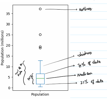
• Box plots:
  • These are based on the percentile we discussed above.
  • The plot indicates outliers, and the 4 quartiles along with the IQR of the data.
  • 
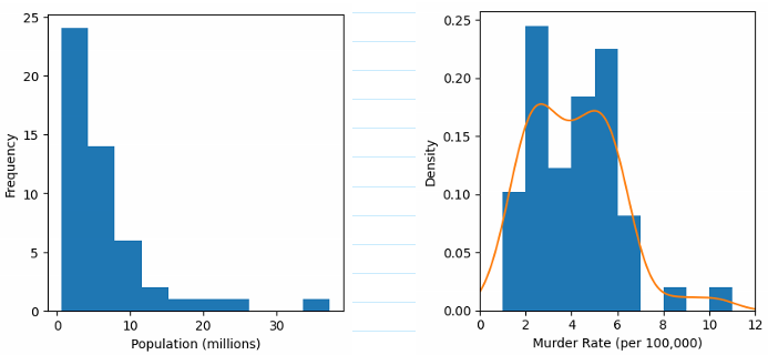
• Frequency tables, histograms and density plots:
  • The data is classified into bins and the count in each bin is called the frequency of the bin.
  • We can use a histogram to visualise the data.
  • For a density plot we can use a ‘kernal density estimate’ to smoothen the histogram

Correlation:

• In Exploratory data analysis, one of the important concept is to check for correlation.
• Correlation is measuring the relation between two predictors or between predictor and target.
• Say two features x,y. How does y change when the x changes. This measure is called correlation.
• Correlation coefficient is metric used to measure the correlation between two features. Its value lies between (-1 and 1). -1 indicates lower correlation and 1 indicating higher correlation between features.
  • Pearson Correlation Coefficient: $\frac{\sum{(x_i-\bar{x})(y_i-\bar{y})}}{(n-1)s_xs_y}$
• When the relation between features are not linear, correlation may not be an important metric.
• This above method of correlation is not robust to outliers.

Exploring two or more variables:

• Some of the plot can be used to explore two or more variables simultaneously.
  1. Contingency table
  2. Hexagonal binning
  3. Contour plots
  4. Violin plot.