Todays topic include:
Matrices
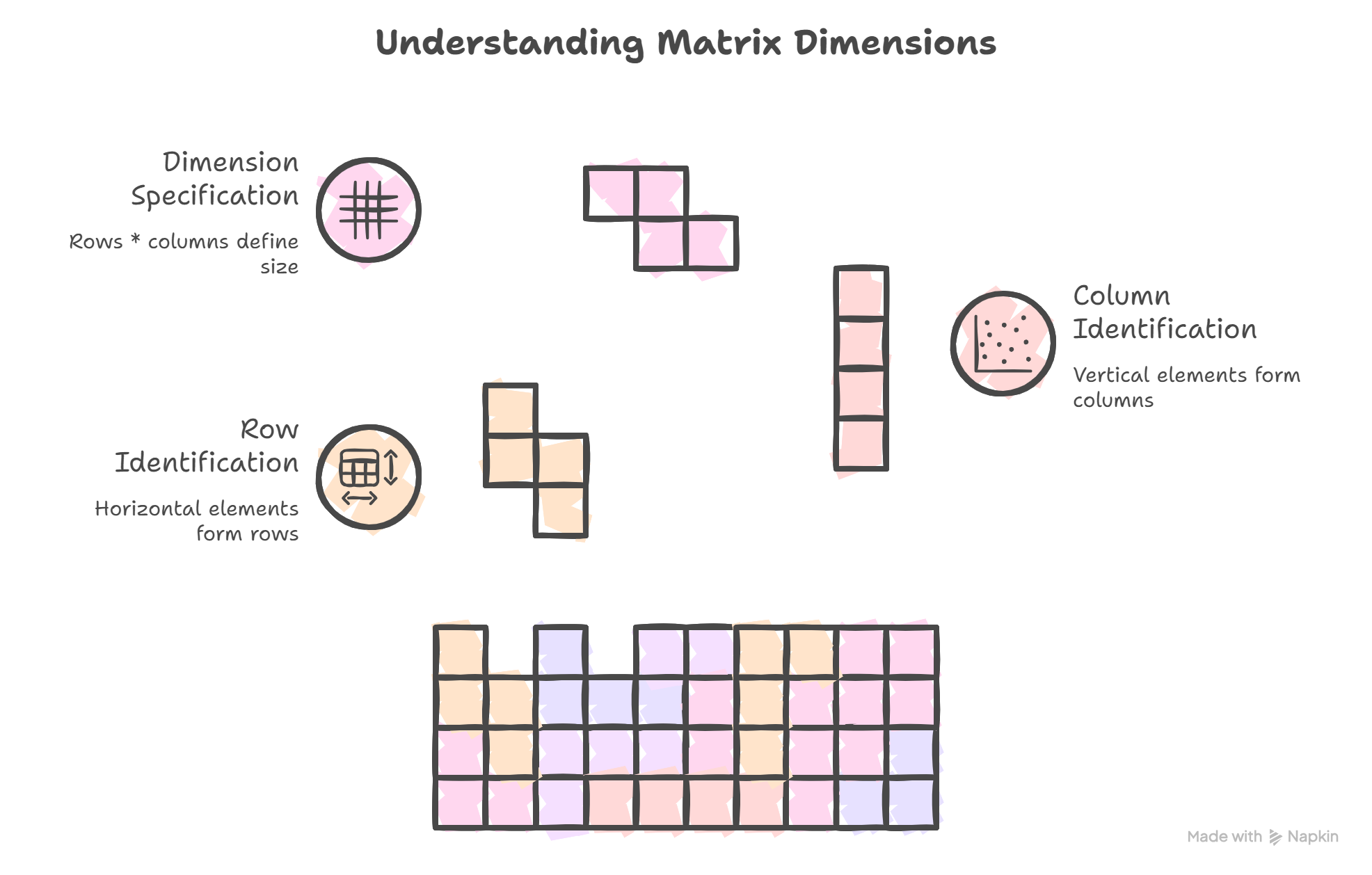
- A matrix is a 2d array of elements. The hoizontal elements are combinedly called as rows. Similarly the vertical elements are combindly called as columns. Using these we can represent a matrix like: A matrix of dimension rows * column.
- The relation between a vector and a matrix can be shortly put as a vector can be transformed using a matrix. For example when a vector is multiplied by a scalar, the vector shrinks or magnifies. In the same way when a vector is multiplied by a matrix, it undergoes certain transformation.
- Example of a matrix with dimension 3*3:
- \[A = \begin{bmatrix} 1&2&3 \\ 4&5&6 \\ 7&8&9 \\ \end{bmatrix}\]
- From the above matrix The column vectors becomes \(\begin{bmatrix} 1\\4\\7\\ \end{bmatrix}, \begin{bmatrix} 2\\5\\8\\ \end{bmatrix}, \begin{bmatrix} 3\\6\\9\\ \end{bmatrix}\).
- The row matrixes for A are: \(\begin{bmatrix} 1\\2\\3\\ \end{bmatrix}\) and so on.. Since the row elements are transposed to make it as a vector they are basically the transposed matrixs instead of direct matrices.
- Identity matrix (I):
- Where the diagonal elements are 1
- Zero Matrix:
- Every element in the matrix is zero
- Transpose of a Matrix:
- The transpose if a matrix $A$ is the $A^T$. Where the columns of the matrix A are the rows in matrix $A^T$
- Symmetric matrix:
- Where $A = A^T$
- Matrix Operations:
- The matrices can perfrom operations like:
- Multiplication by scalar
- Matrix addition
- Matrix-Matrix multiplication
- When two matrices (mn, jk) are multiplied, it produces another matrix of size (m*k). The matrix operation can only be carried out only if n =j. $(m \times n)\times (j \times k) = (m \times k) \iff n = j $
- Matrix subtarction can subtraction can be performed by using the 2&3 like $C = A+(-1)B$
- The matrices can perfrom operations like:
- The dot product can be performed using matrix multiplication:
- \[u \cdot v = u^T\cdot v = (u_1, u_2 ...) \begin{pmatrix}v_1\\v_2\\.\\.\\.\\ \end{pmatrix} = \sum_{i = 1}^n u_iv_i\]
- Matrix Inversion:
- When we have an equation to solve: Ax = b, How do we solve it?
- We can use matrix inversion:
- Check if the matrix is inversible (Only square matrices can have Inversions)
- Calculate the inverse of matrix A
- Multiply ‘b’ by the inverse of A $(A^{-1})$
- Verify the solution
- A Square matrix A is said to be inversible when there exists a matrix $A^{-1}$ such that: $A \cdot A^-1 = I$
- The inverse of a $2\times2$ matrix is given by:
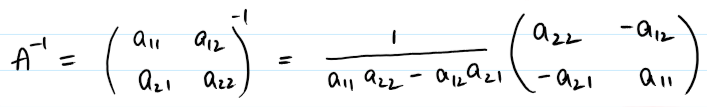
- The denominator is also called as the determinant of the matrix.
- The matrix A is said to be linearly independent if $AX=0$. Meaning the solution is trivial.
- A matrix is linearly independent if no column in the matrix can be expressed as a linear combination of other columns. If there is one other solution other than AX=0, the matrix A is linearly dependent
- Basis theorem states that,
- In a 2D plane two vectors, u,v form a basis if u,v are linearly independent
- In a 3D space, the three vector u,v,w must be linearly independent to be a basis of the 3d space.
- In 2D and 3D spaces, there are some matrices used for Rotation, Shearing and Scaling a vector. When multiplied by these vectors, we can perform the intended operation on the vector But what happens when there are two different coordinate systems?
- When there are two different basis (say two different coordinate systems with different bases), we can formulate a matrix such that we can represent any vector in one basis to another basis
- $v = B\hat{v}$
- Where v is the vector in one basis and $\hat{v}$ is vector in another basis. The matrix B can be used to transoform one coordinate to another. This is core concept used in coordinate transformation in robots, image processing and many more.
- Orthogonal matrix:
- A matrix Q is said to be orthogonal if its transpose is its inverse matrix.
- \[Q^{-1}\cdot Q^T =I \iff Q^{-1}=Q^T\]
- So, an orthogonal matrix is a square matrix with the column vectors perpendicular to each other and one unit long.
- An orthogonal matrix will rotate a vector in a 2D space but will not cause shear or strech.
- A matrix Q is said to be orthogonal if its transpose is its inverse matrix.
Determinants:
- The denominator in the inverse of the matrix is called as determinant of the matrix.
- This is very useful for determining the properties of a matrix like if the matrix is invertable (if $det(A)=0$), if a linear equation has a unique solution or no and so on..
- $det(A) = 0$ has only one unique solution
- $det(A) \ne 0$ has many solutions
- For a matrix A of dimension $(3 \times 3)$ the determinant is defined by det(A) or $|A|$ and is given by:
- \[det(A) = \begin{vmatrix} a_{11}&a_{12} \\ a_{21}&a_{22} \end{vmatrix} = a_{11}a_{22}-a_{12}a_{21}\]
- similarly we can get the determinant for higher dimension matrices just like the cross product
- Some useful properties of determinant:
-$det(A) = det(A^T)$
- $det(AB) = det(A)det(B)$
- Adjoint Matrix:
- Adjoint matrix is useful for finding the inverse of a matrix without the complex formula as seen before for smaller matrices $2 \times 2; 3 \times 3$
- \[A^{-1} = \frac{1}{det(A)} \cdot adj(A)\]
- Cramer’s Rule:
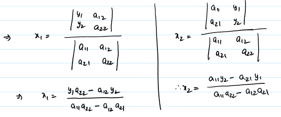
- Crammers rule gives an explicit formulae for solving a system of equations or say a linear equation Ax = y, without needing to find the $A^{-1}$ given that the $det(A) \neg 0$
- All the values of $x$ are then given by just dividing the determinants of a modified matrix ($A_i$) with the determinant of A
- $x_i = \frac{det(A_i)}{det(A)}$
- Where $A_i$ is obtained by replacing the $i^{th}$ column in A with the constants in y
- Therefore: $x_1 = \frac{det(A_1)}{det(A)}; x_2 = \frac{det(A_2)}{det(A)}$
Gaussian Elimination:
- Gaussian Elimination is a method to solve the system of linear equations.
- As we will see in the following section, that Gaussian elimination can also result in other fruit full outcomes like finding the rank, nullity of the matrix. These are some of the useful properties of the matrix describing how solid the matrix is.
- Gaussian Eliminatopn does not chang the rank, column space or null space of the matrix. It just strips the excess information from the matrix
- The basic idea of Gaussian Elimination is to do some row operations to make to make the matrix into something called Row Echelon Form (REF) or further Reduced Row Echelon Form (RREF).
- Swapping the rows : We can swap any two rows
- Scaling the rows : A row can be multiplied by a non zero scalar
- Row Addition : Two rows can be added, subtracted to find the pivot element
- The REF form of the matrix has all the zero rows at the bottom and non zero rows at the top.
- We end the row operations when we found the pivot elements for each non zero row to achieve REF.
- For example:
- \(A = \begin{bmatrix} 1&2 \\ 3&8 \end{bmatrix}\) can be written into its REF \(\begin{bmatrix} \underline{1}&2 \\ 0&\underline{2} \end{bmatrix}\) by performing $\to R_2-(R_1 \times 3)$.
- The underlined elements are the pivot elements of that row. See how the row elements are 0 before the pivot elements?
- It can further be reduced into its RREF by $\to \frac{R_2}{2}$ so that all the pivot elements would be 1, to become \(\begin{bmatrix} \underline{1}&2 \\ 0&\underline{1} \end{bmatrix}\)
- The solution of the Gaussian elimination caould be either
- Has one solution for the system of equations (The lines in the System of equations intersect at 1 point)
- Has No solution (The lines could be parallel lines so, no solution)
- Has infinit solutions (the intersection could be a line, plane,..)
Rank:
- Rank is a property of a matrix that truly tells how much information is in the matrix.
- It is the number of linearly independent columns or rows in a matrix. Full rank is when the rank of an $n \times n$ is n, if the rank is less than n then it is called rank deficit. A full rank matrix is a solid rank without any redundant informantion. Rank deficit means that the matrix has some redundant information.
- The matrix like \(\textbf{A} = \begin{bmatrix} 1&2 \\ 2&4 \end{bmatrix}\) has a rank of 1. This matrix when applied to a 2D space, it will collapse everyting to a 1D space. This property is useful in some cases where we need to reduce the diminsionality of vector space.
- A rank of the matrix can be found out after transforming the matrix to its REF.
- Nullity:
- Also an important concept is the Nullity of the matrix, $Rank(A) + Nullity(A) = number of rows(n)$. As seen above, the number of dimensions that were collapsed during the transformation is the nullity of the matrix.
- Nullity is the dimension of the nullspace of the matrix.
- In datascience this helps to identify the features that are redundant and add no new information for the model during training.
- Null space:
- The Null space of A is the entire solution set for the $Ax = 0$.
- To find the Nullity of a matrix, we can use the RREF and in this form, the number of rows with the pivot elements are the Rank of the matrix and the number of rows with no pivot elements are the nullity of the matrix. This should make sense with the above equation.
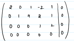
- For example for the below REF form of a matrix, there are 2 columns that are either zero or without pivot element. So the rank is 3 and nullity is 2.
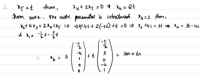
- Therefore the above solution is the nullspace of the matrix A.
- Row Space and Column Space:
- The set of all linear combinations of the linearly independent columns or rows of the matrix are called the column space or rowspace of the matrix.
- The number of linearly independent rows or columns are also called as Row rank (rowrank(A)) and Column rank (colrank(A)) and can be otained from the REF. It can be observed that the row rank and column rank are equal to rank of the matrix.
- The columns and rows of the pivot element form the basis of the column space and row space respectively.
- For a product of two matrices $A=BC; rank(A) \le rank(B) \& rank(A) \le rank(C)$.
- These concepts are also used by Singular Value Decomposition(SVD) used in AI and other technologies.