It would be nice to revisit calculus while I’m at revisiting the math backgrounds. So, todays blog is related to calculus Todays topic include:
Calculus is made up of mostly two symbols:
- “d” meaning 'A little bit of', when someting says “dx” it means little bit of x. Usually indefinitly small pieces. Called as Differential
- Remember when $dx$ is itself infinitly small, the higher order terms would be even smaller. So for many calculations the higher order terms are generally omitted to make the calculations simpler.
- ”$\int$” meaning 'the sum of', when we see “$\int{dx}$” it means sum of all the little pieces of ‘x’. Called as Integral
Differentials:
- Suppose there is a ladder that was laid against a wall. Say the reach of the ladder horizontally as ‘x’ and vertically as ‘y’.
- What happens to ‘x & y’ when the ladder’s tilt is changed a little bit?
- Say the horizontal reach is changed a ‘little bit’ say ‘dx’ and vertical ‘dy’.
- The change in vertical reach (dy) might be positive or negative based on the change in the horizontal reach(dx).
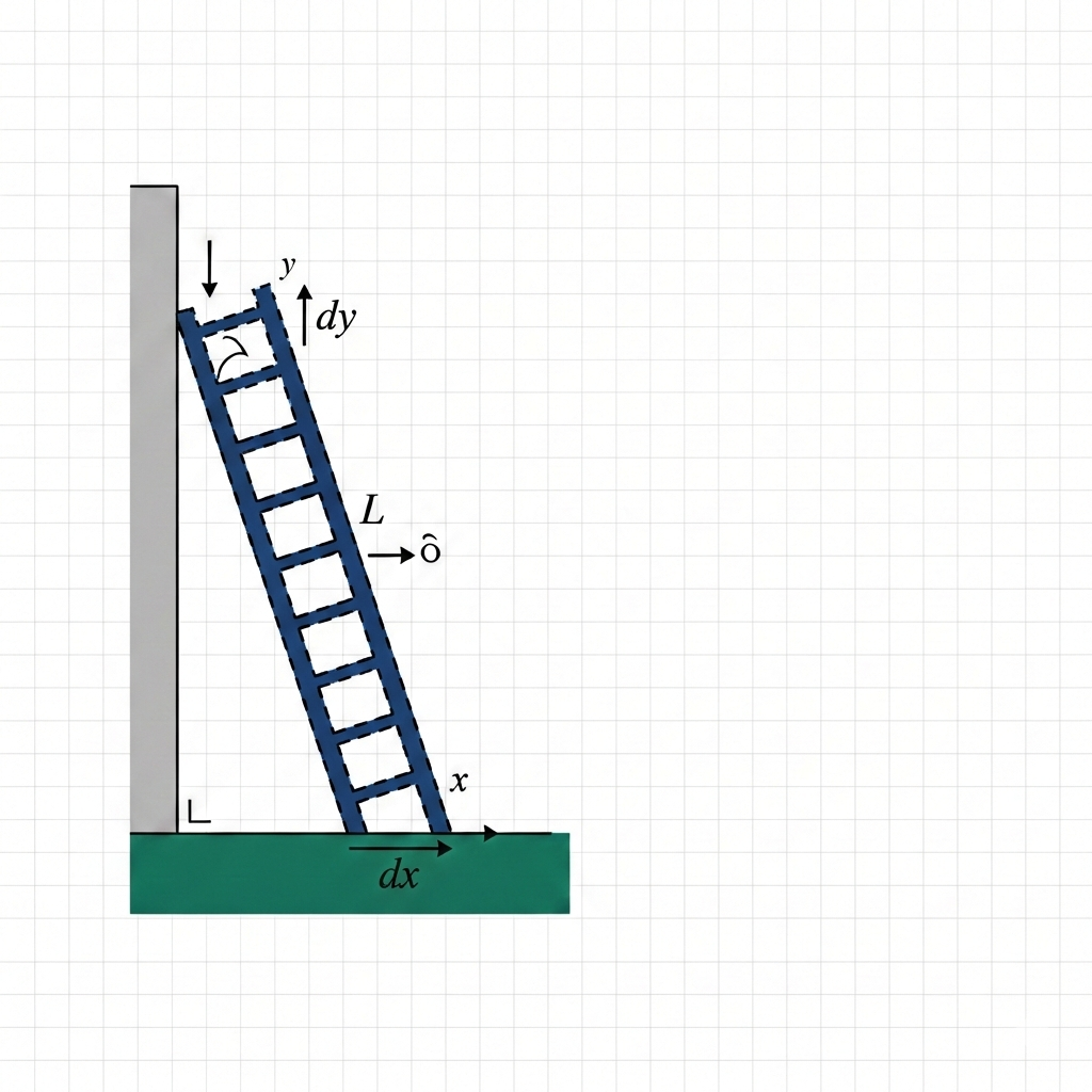
- The goal of the differential equation is to find the ratio $\frac{dy}{dx}$ (differential coefficient of y wrt x). The change in vertical reach with respect to the change in the horizontal reach!!
- $l^2 = x^2+y^2$ type of functions are called Implicit functions that has this dependency implicitly inside the function and are represented by the form $F(x,y)$.
- The other form of functions are the explicit functions, like for the ladder example we can say that $y = \sqrt{l^2-x^2}$ as it forms a right angle triangle, in which the variable ‘y’ is called dependent variable which depends on the variable ‘x’(Independent variabe). We can write this in the form $y =F(x)$
- Also when a function is differentiated($F(x)$) can be represented as $F’(x)$ equivalent to $\frac{d(F(x))}{dx}$.
- This is called as ‘derived function’
- Added Constants in the differential equation does not change the end result. Howver Multiplied constants multiply the end result
- Example: $y = x+2$ and $y = 2x$
- Sums and differences:
- When we need to find the differential coefficient of the sum of two functions of x, for eg: $y=(x^2+c)+(ax^4+b)$. This is quite simple, just differentiate the two equns one after the other. The ans will be $dy/dx=2x+4ax^3$.
- The solution for $y = u+v$: $\frac{dy}{dx}=\frac{du}{dx}+\frac{dv}{dx}$
- Products:
- The product of two equations is not a straight forward thing as we have seen in constants section that a constant multiplied to a function can have an impact on the final result. Eg: $y=(x^2+c)∗(ax^4+b)$
- The solution for $y = u\times v$ will be: $\frac{dy}{dx}= u \cdot \frac{dv}{dx}+ v \cdot \frac{du}{dx}$
- Quotients:
- For $y = \frac{u}{v}$, the solution will be: $\frac{dy}{dx}= \frac{(v \cdot\frac{du}{dx}−u \cdot \frac{dv}{dx})}{v^2}$
- Successive Differentiation:
- A function can be differentiated succesively., the second time a function is differentiate is called ‘second derived function’ and so on..
They can be represented as before but with two dashes $F’‘(x) = \frac{d(\frac{dy}{dx})}{dx}$
- For example when the distance is differentiated wrt time, we get velocity. Which gives acceleration when differentiated again!! This differentiation wrt time has a word called rate. The rate of change of some thing…
- let ‘y’ be the distance and velocity $\nu = \frac{dy}{dt}$ and acceleration is $a = \frac{d(\frac{dy}{dt})}{dt}$
Geometric meaning:
- Well, what is the real importance of differentiation? We can explain this using a graph.
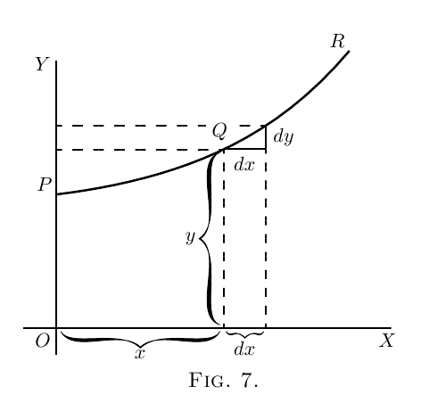
- Imagine the graph above shows the curve. Take a small piece of the curve and we can say that dx is the small change in x axis and dy would be the small change in the yaxis. When we find the ration $\frac{dy}{dx}$ when the observed curve is infintly small, we can consider it as a straight line. Now this ration can be treated as the slope of the curve at that point.
So the ratio $\frac{dy}{dx}$ gives the slope of the curve at a particular point in the curve.
- This value (differential coefficient) says a lot about how the curve behaves at that point of the curve.
- The value is 1, means that the curve is slopping at $45^0$
- The value greater than 1 meaning the curve has a slope more than $45^0$
- When the value is negative, the slope is curving downwards.
- The value is increasing, the curve slope is increasing
- Similarly, the slope decresing meaning, the curve is gradually approaching horizontal nature(not untill 0)
- But an interesting case appears, when this value becomes 0. This means that the curve doesnt have any slope meaning it is horizontal. This horizontal appears only in two cases for a curve. Maxima and a Minima.
- Maixma and Minima:
- One of the main reasons to differentiate a function is to findout where or if the curve achieves its maximum value or minimum value. This is an important concept in Engineering and AI to maximize the efficieny of a model.
- So, when modeling the function could be differentiated and equated to zero. Now solve the equation to find the point where the maximum or minimum is present.
- But One problem is we do not know if the point belongs to a maxima or a minima?? It just tells where the slope of the curve is 0
- This is where successive differentiation comes, when find a second derived function, we can determine if the point belongs to a maxima or a minima! How??
- The value $F’‘(x)$ gives the ‘curvature of the slope’
- Well, When the slope($F’(x)$) is constant, the value of $F’‘(x)$ becomes zero.
- When the slope is increasing, the $F’‘(x)$ value increases
- when the slope is decreasing, the $F’‘(x)$value decreases.
- We can use this sign to determine if the point is a maxima or a minima.
- When the value $F’‘(x)$ is positive, we can say that the point at which $F’(x)=0$ is a Minima
- When the value $F’‘(x)$ is Negative, we can say that the point at which $F’(x)=0$ is a Maxima
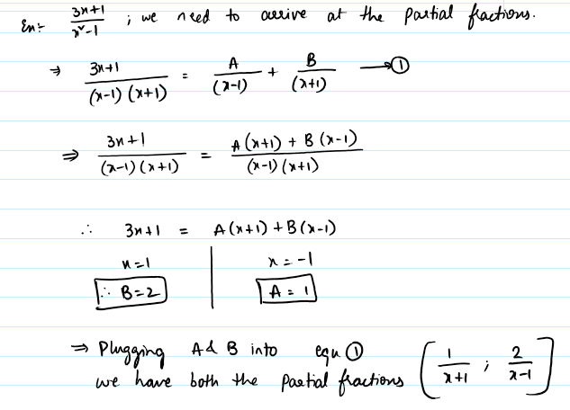
Partial fractions:
- When the function(fraction) is to complicated to differentiate, we can decompose the fraction into smaller functions and work with them
- for example:
Partial Differentiation:
- What do we do when the function contains more that one independent variable like $F(u,v)$?
- we can now use partial differentiation to differentiate the function.
- We first consider one variable to be constant, say v as constant! Then $dy_v=v.du$
- Similarly next of u is considered constant then $dy_u=u.dv$
- Since the differentiation has been partially performed on the equ, the above equations are also called as partial differentials. They can also be written as:
- $\frac{\partial{y}}{\partial{u}}=v$ and $\frac{\partial{y}}{\partial{v}}=u$
- Substituting these in above equns:
- $dy_v=\frac{\partial{y}}{\partial{u}} \cdot du$ ;and $dy_u=\frac{\partial{y}}{\partial{v}} \cdot dv$
- Since the y depends both on u, v. To achieve total differential we add both the terms above which leads to:
- $dy= \frac{\partial{y}}{\partial{u}}\cdot du+ \frac{\partial{y}}{\partial{v}} \cdot dv$
Integration:
- As already said, integral is the sum of. When we say, $\int dx$ then that should make the whole of ‘x’.
- Now, we can ask the question if we have the slope of the curve given can we recreate the curve.
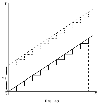
- For example take a line we have the equation $y = ax+b$, the slope is ‘a’ and the y-intercept ‘b’.
- This slope $\frac{dy}{dx} = a$, this says the small triangles that are under the curve. Now when we stack those triangles together we can form a line. But the intercept is missing we do not have any knowledge about it, where do we place the y-intercept?
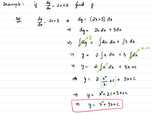
- To tackel this intercept we add a constant term ‘C’ after integrating!
- What happens if it is a curve. We then have the slope as a function of ‘x’ like $\frac{dy}{dx}= ax$. As the value of x increases, the slope increases.
- The problem is when the triangles are not small, the curve would be a coarse. If the curve needs to be sommther, the triangles need to be as small as possible.
- Integrations can also be used to find the areas under the curve. The area under curve, can be divided into strips. Each strip can be considered as a rectangle and all the strip can be integrated to find the area under the curve. This is where the bounds come.
- As a curve can be extended limitless, we find the area of the curve bound by Limits. They were upper and lower bounds. They can be represented as $\int_{x=x_1}^{x=x_2} y.dx$